Similar articles

Abstract: We solve the problem of petroleum products distribution through oil pipelines networks. This problem is modelled and solved using two techniques: A heuristic method like a multiobjective evolutionary algorithm and Mathematical Programming. In the multiobjective evolutionary algorithm, several objective functions are defined to express the goals of the solutions as well as the preferences among them. Some constraints are included as hard objective functions and some are evaluated through a repairing function to avoid infeasible solutions. In the Mathematical Programming approach the multiobjective optimization is solved using the Constraint Method in Mixed Integer Linear Programming. Some constraints of the mathematical model are nonlinear, so they are linearized. The results obtained with both methods for one concrete network are presented. They are compared with a hybrid solution, where we use the results obtained by Mathematical Programming as the seed of the evolutionary algorithm.

.  INTRODUCTION

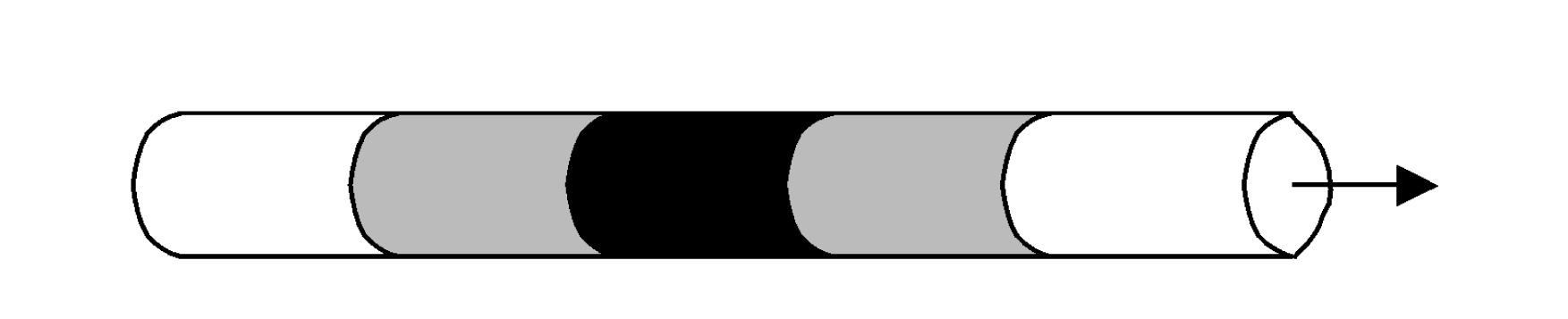
 Polyducts are pipeline networks designed to transport oil derived products. Unlike conventional pipelines, which transport only crude oil, polyducts transport a great variety of fuels treated in refineries: kerosene, naphthas, gas oil, etc. Transport is carried out in successive packages as shown in Fig.1. A package is a changeable quantity of the same product class located along a polyduct. A long polyduct can contain four or five different products each occupying respective extensions along its route. The entry points and supply sources of the polyducts usually receive products directly from refineries or ports where ships coming from refineries unload. The delivery points are receipt terminals or intermediate stations with storage tanks located along the route. Providing that certain constraints are fulfilled in the package arrangement, the mixing of successive products affects only a minimal fraction, and the mixed products can be recovered as low quality product.




 The polyducts in a specific geographical area (region, country, etc.) are interlinked to form polyduct pipelines. To move the products, pumps are distributed strategically along the network. From an operative point of view, a polyduct network will be constituted by a set of nodes with storage capacity, and a set of edges (the polyducts) which interconnect the nodes. The edges are mostly unidirectional, but for reasons of operative flexibility, there can also be bidirectional edges. The network topology can be very varied, depending on the oil activity and geographical region conditions. The nodes, in general, will have the capacity to supply, store and receive products (De la Cruz et al., 2004).

 On a logistic level, the problem of polyduct pipelines is to plan the way different products are temporarily transported from source nodes to demand nodes, passing through intermediate nodes. Planning must satisfy a set of temporary constraints, related to the minimum and maximum dates for the delivery of different products. Also, constraints related to the products at the sources availability must be dealt with and the proper physical conditions after network utilization must be satisfied. The quality of the solutions to these problems is usually measured in terms of minimization of planning time, and the appropriate arrangement of the successive packages to obtain interfaces without mixing. This quality measurement is usually formulated as a multiobjective function of an optimization problem (Chankong and Haimes, 1983). The storage capacity of the intermediate nodes can be used as a strategic element in dealing with temporary constraints and the optimization of the overall objective function. For example, a product that must be transported from a distant supply source to a final node through an edge that is being used at the time for another shipment is sent to an intermediate node, and then resumes its journey to its destination as soon as the mentioned edge is free.

 In this paper we present a solution to a simplified problem of the optimal distribution of products through pipeline networks using two methods, namely, Multiobjective Evolutionary Algorithm (MOEA) (Goldberg, 1989; Michalewicz, 1995) and Mixed Integer Linear Programming (MILP) (Marriott and Stuckey, 1998; Bazaraa et al., 1990). In Section 2 we study the model of the problem. In Sections 3 and 4 the model representation is given in MOEA and MILP, respectively. An example is solved and compared with a hybrid solution in Section 5. The conclusions are stated in Section 6.

.  MODEL OF THE NETWORK

 We consider a simplified model of an actual network. The network has a set of nodes made up of a set of sources, a set of sinks or receiving terminals, such as delivery points or storage terminals, and a set of intermediate connections serving as receiving and delivering points with storage capacity.

 Every source and intermediate connections may have different polyducts to different nodes and can deliver different products in different polyducts simultaneously.

 We consider that the different products are delivered as discrete packages. There might be as many different types of packages as the number of different products. A unit package is the minimum fluid volume delivered by a source or intermediate node in unit time. Every sink and intermediate node have as many tanks as products it can receive, to store the different products. Also we can assume that the sources take the fluids from tanks. In order to simplify the problem we assume that all polyducts have the same diameter and characteristics.

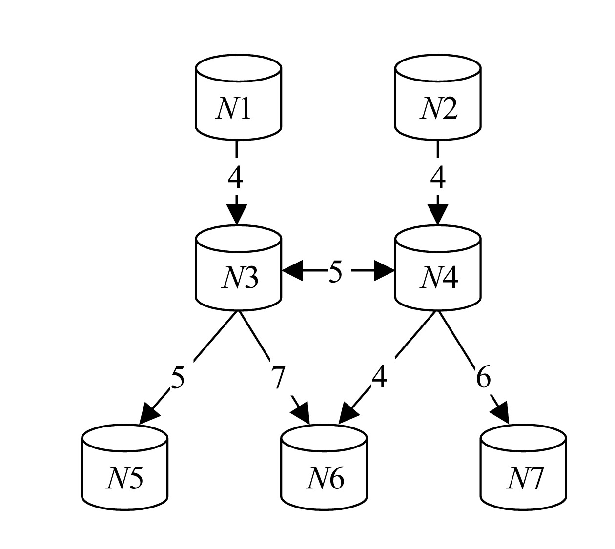
 We also assume that all packages flow with the same speed and that they occupy a similar volume in the polyduct. If two packages of different fluids follow one another there exists the possibility of both products becoming contaminated. In a number of polyducts the fluids may flow in both directions from one node to the other. One of the studied networks can be seen in Fig.2. This network has two sources (N1 and N2), three sinks (N5, N6 and N7) and two intermediate nodes (N3 and N4). In the polyduct joining nodes N3 and N4 the fluid can flow in both directions. Numbers in links joining two nodes give the normalized distance in terms of units of time needed by a given package to cover the whole polyduct. For instance, number 7 in the polyduct linking nodes N3 and N6 means that one package spends seven periods of unit time to go from node N3 to node N6, or that the polyduct may contain seven packets.

.  HEURISTIC METHOD

 We describe the data structure, operators and functions that characterize the solution space. First we present the solution coding and then we describe the most important genetic operators used over the population.

 To code the topology of the network we use a matrix having as entries the distance among the nodes (Botros et al., 2004). An entry of zero means there is no connection between these nodes. A connection is represented as a pair (i, j) where i is the output node and j the input node. A bidirectional links is acknowledge because we have a pair of symmetric connections (i, j) and (j, i).

.  Coding a solution

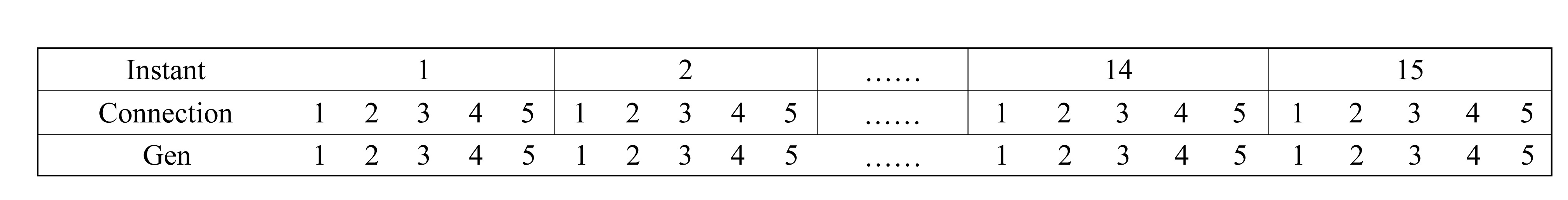
 A solution to the problem is given by the kind of packet sent by every source or interconnection node at every instant (De la Cruz et al., 2003). To code a solution we use a matrix to represent the population, with a row for every individual as shown in Fig.3. For each individual the first n elements store the types of package units sent through the n connections in the first instant of time, the following n elements the types of package units sent during the second instant of time, and so on.




 However, this codification does not necessarily fulfil the problem statement conditions yet, because the product type produced for each source could be different, and all the elements in the row vector solution are in the range [0, number of product types]. The easiest way to handle this aspect of the problem is to code, for each source, the types of oils from 1 to the number of different oils sent by that source (leaving the 0 for the case of not sending any product at that instant of time). This coding will not overload the genetic operators and the real type of oil coded in the individual must be obtained, before evaluating the individuals to obtain their fitness, by means of the ProductType variable.

 For example, for the network of Fig.2, if the source 1 can handle packages of types 1 and 2, and the source 2 can handle packages of types 3 and 4, the valid values in the individual row vector for the connections 1 and 2 will be in the range [0, 2] and for the others in the range [0, 4]. In the two first connections, the values 1 and 2 will code types 1 and 2, while in the second the same values will code the types 3 and 4. For all the other connections, the values [1, 4] will code types [1, 4].

 This information coding can be kept easily in a structure where every row is a cell associated with a node, and within every row, there are as many columns as connections departing from this node. So the value of the gene acts as entry to get the product associated with it. In Matlab notation the representation of this information is as follows:

 ProductType={[1 2];

 [3 4];

 [1 2 3 4];

 [1 2 3 4]}

 With this representation the products associated with the genes of the first node are:

 ProductType {1}(1)=1;

 ProductType {1}(2)=2;

 and those of the second node are

 ProductType {2}(1)=3;

 ProductType {2}(2)=4;

 and so on.

.  Genetic operators

 For the generating process, we can build a mask in order to keep each gene of our individual structure (type of package sent by each connection in each time instant) in its corresponding value range. An example is given in Table 1, where Mask is a vector which contains in each entry the number of different products that can be sent by each connection.




 Then, if we have Nind=20 individuals (with 8 connections and 15 time instants) we can use the mask to generate the initial population as follows (using Matlab notation):

 Nconex=8;

 Ninst=15;

 Ngenes=Ninst*Nconex;

 Nind=20;

 mask=[2 2 4 4 4 4 4 4];

 pop_aux=rand(Nind,Ngenes);

 mask=repmat(mask,Nind,Ninst);

 pop=round(pop_aux.*mascara);

 Now, we explain the genetic operators used in the reproduction process:

.  1. Crossover operator

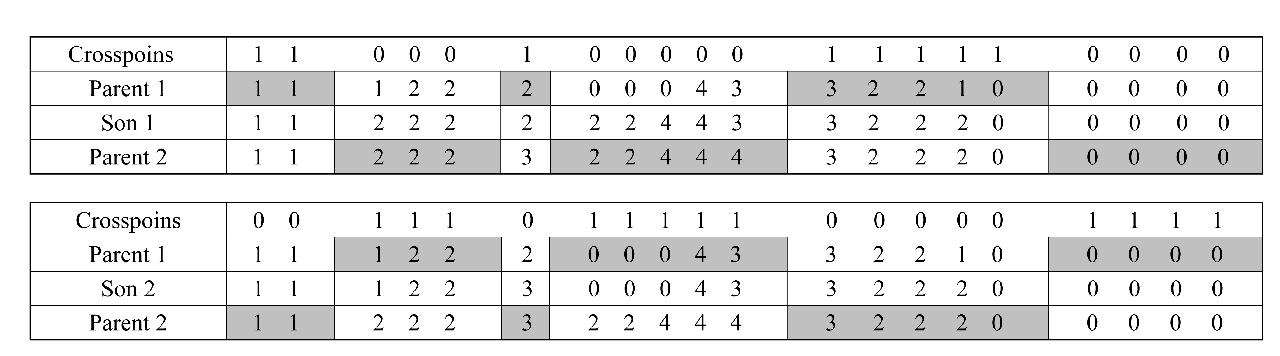
 A uniform cross point function is used to select randomly the crossover points for each pair of individuals of two genetic populations. The crossing points CROSS POINTS are returned in a numeric matrix of 0 and 1 with as many rows as pair of individuals and columns as number of genes. The crossing points are identified as the points where there is a change from 0 to 1 and from 1 to 0. So, if the number of crossing points is n, each row has n+1 string of continuous values (0 or 1). Fig.4 is a schematic of such cross method with n=5. In our case we adopted n=2.

.  2. Mutation operator

 Again we can use the mask to implement the mutation operator. Continuing with the above example the implementation of this operator with Matlab notation is:

 probMut=0.008;

 mutp=(rand(Nind,Ngenes)
 pop_aux=rand(Nind,Ngenes);

 mutated=round(mask.*pop_aux).*mutp;

 new_pop=pop.*(˜mutp) + mutated;

.  Design problem

 In addition to satisfying the demands in time, the main objective is to reduce to a minimum the number of different kind of packets through every pipe, so that to avoid, as much as possible, the possibilities of contaminating products, while verifying a number of constraints for every time interval used to solve the problem. The working strategies obtained with the genetic operators designed are not always feasible, so the MOEA must deal with the existence of invalid solutions. The implemented MOEA uses a repairing operator to modify those individuals which violate the tanks capacities, and/or which have packages arriving outside the limits of time, and/or whose destination points have received more package units than requested. The remaining constraints are used in the evaluation step to rank the individuals, penalizing the fitness of those individuals which does not fulfil them. To do that, we can consider the following objectives and constraints used by the MOEA.

 The constraints are as follows:

 It is necessary to satisfy a minimal production: (1)

 P_ij is the minimum number of packets of product j to be sent from source I; E_ij is the number of products j that has been sent to it by source I; UbC_ij is the upper limit in number of packets of tank j of node I; Nf is the number of source nodes; and Nti is the number of tanks in node i, i.e., number of products. A solution to the problem is penalized depending on the degree of satisfaction of such restriction by the constraint J₁.

 The tank capacity must not be violated: (2)

 packets of tank j for node i, and Ni is the number of intermediate nodes. A repairing function can check if each package sent violates the lower capacity of the source tanks and eliminate it from the chromosome via repairing operator R₁ if it happens. Nothing can be repaired for the upper limit of the arrival tanks because we do not know the future state of these tanks. Then, the degree of complying with such restriction can be measured by J₂ in the objective function. This represents the balance.

 Every destination must receive the amount of demanded packets: (3)

 destination i, D_ij is the number of packets of product j and Nd is the set of nodes with a certain demand. A solution to the problem is penalized depending on the degree of compliance with such restriction indicated by the constraint J₃. In addition, a repairing function is employed to eliminate of the chromosome the additional packages that surpass the number of requested packets by repairing operator R₂.

 There must be no collisions of packets through a bidirectional pipe: (4)

 NC is the number of collisions in bidirectional pipes. This restriction is verified with objective function J₄. A solution to the problem is penalized depending on the degree of accompliance with such restriction.

 The arrival of a packet to a node must be at due time: (5)

 LbT_i (UbT_i) is the lower (upper) limit in the arrival time of packets to destination i and T_i is the time of arrival of a packet of any product to destination i. Whenever a package is sent, it is verified if it complies with this restriction. In affirmative case the sending of this package stays in the chromosome and in the opposite case it is eliminated via repairing operator R₃. Applying this function on each one of the sent packages ensures compliance with this restriction at every moment.

 The objectives are as follows:

 Minimize the number of product changes, or fragmentation: (6)

 Minimize the time it takes to verify the demand: (7)

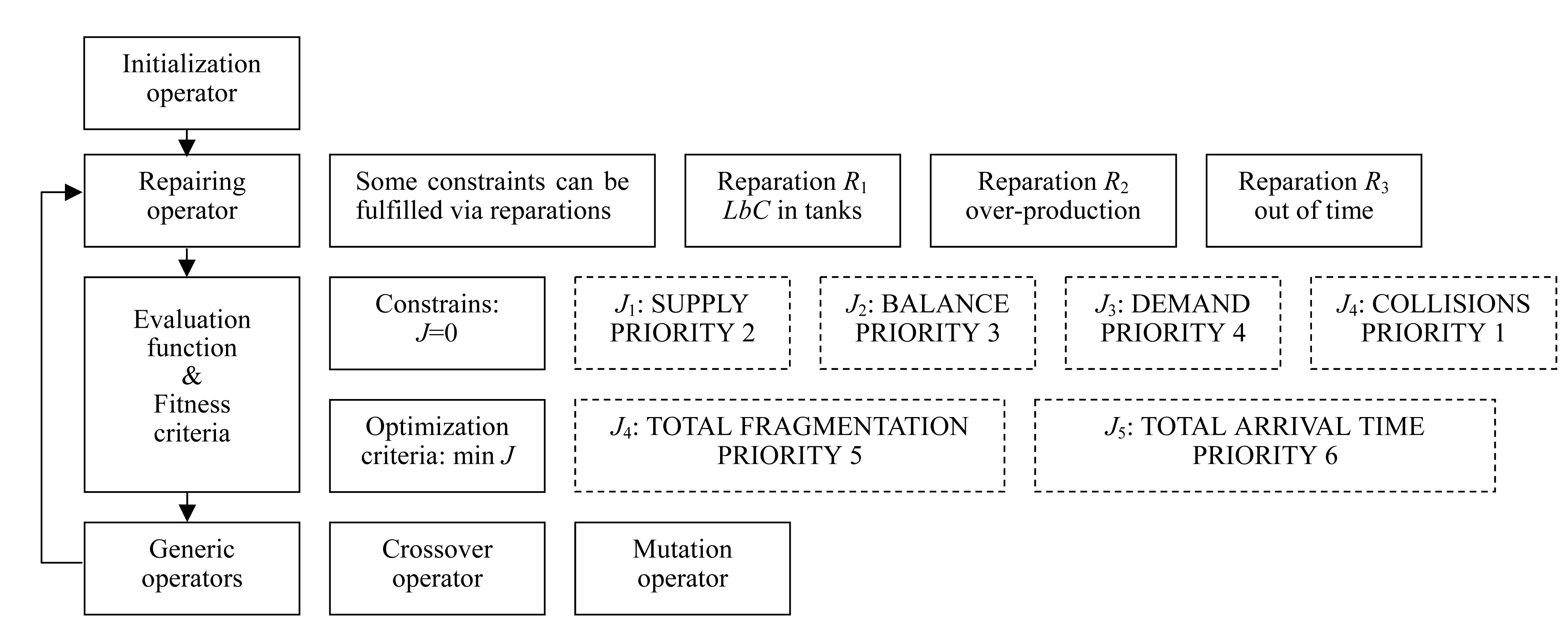
 The MOEA implemented is schematised in Fig.5 showing the flow diagram of the modules included in the algorithm with their corresponding functionality.

Fig.6
Constraints satisfaction in MOEA

 The algorithm begins with the creation of an initial population. Next some repairs are applied to these individuals and then the objective functions are evaluated and the population is ranked using the priority parameter given in Fig.5. Now a dominance matrix is built. This matrix keeps the dominance relation between each pair of individuals. Fitness is assigned over the population using Goldberg method (Goldberg, 1989; Michalewicz, 1995). In this method the population is divided into several groups. First, a group with individuals that are not dominated is formed; next, a group is obtained by eliminating from the population the individuals from the first group and taking the individuals that are dominated, and so on. The individuals in a group are given the same fitness value. The worst group is given a fitness value of 1, the second worst group is given a fitness value of 1+Δ, the third worst group is given a fitness value of 1+2Δ, and so on. Δ is a design parameter. The fitness value given to every group with the objectives values obtained by each individual gives the final value used for selecting the parents. With these fitness the MOEA selected the parents for the recombination process and applied the genetic operators to obtain a new population for the next generation.

 Finally we explain the priority scheme. The objective functions for each population are evaluated, and the population is ranked using the preferability relation given in Fig.5 through the priority parameter. Since the algorithm does not repair collisions in bidirectional pipes, the priority of J₄ must be set to 1. Moreover we set priority 2 for J₁, which forces solutions to send all the supply. Next we want to balance the intermediate nodes (priority 3 for J₂) and all the demanded products must arrive at their destinations (priority 4 for J₃). While the previous constraints are not complied with, we do not evaluate the objective functions; for this reason the priorities of J₅ (fragmentation) and J₆ (maximum arrival time) are set to 5 and 6 respectively.

.  MATHEMATICAL PROGRAMMING

 The polyduct pipelines in this study can be represented initially by a set of nodes, edges (polyducts) and product types R=⟨N,C,P⟩, and whose activity is determined by a time interval T. Demand must be

 satisfied in this time interval. For the network components N is the set of network nodes, where N_D is the set of nodes with a certain demand. C=C_U∪C_B is the set of network edges, where C_U is the set of unidirectional edges and C_B is the set of bidirectional edges. P is the set of product types to be distributed in the polyducts.

 For the system variables and system parameters, a is defined as a store variable, indexed in time, node and product ⟨t,n,p⟩. Its lower and upper limits are denoted as a^inf and a^sup respectively. s is the transport variable, indexed in time, origin, destination and product ⟨t,n₁,n₂,p⟩, and represents the quantity of product that flows from the point of origin to the destination within the specified time. Its lower and upper limits are s^inf and s^sup respectively. ||n₁,n₂|| defines the edge sections that join both network nodes; provided that a product p crosses a section for a time unit; this quantity indicates the time units that the products take to cross the polyduct and the edge.

 Auxiliary variables are needed to determine the different changes of product type that is made in each polyduct. In this way, δ, indexed for time, origin, destiny and product, is defined. It represents whether or not the product is transported within its index, taking values one and zero in each case. Nevertheless, given the transport normalization for amounts, it is assumed that δ≡s. In addition c is indexed in time, origin and destination, and counts the product changes produced in the edge in the time interval [0, time_index].

 For constraint problem modelling, the standard network topology constraints are defined first, i.e., node balances in nodes and edge limits, later adding other dependent constraints directly to the treated problem characteristics, since they might be the product changes or conditions derived from polyduct bidirectionality (Magatão et al., 2004).

 In this case, the problem constraints can be classified by examining their linearity or nonlinearity (Schrijver, 1986; Luenberger, 1984).

.  Linear constraints

 First, the storage constraint is presented. For each t∈T, n∈N, p∈P it is required that (8)

 Secondly, the balance constraint is defined in every network node, i.e., for each t∈T, n∈N, p∈P it is required that (9)

 In the third situation, the maximum and minimum transporting capacities are defined. Provided that the product transport is normalized, for each t∈T, ⟨n₁,n₂⟩∈C, p∈P (10)

 Next, the constraint based on only one product entering a polyduct per time unit is defined, for each t∈T, ⟨n₁,n₂⟩∈C, p∈P (11)

 The fifth point is that it is important to emphasize that a product will not leave the polyduct if it does not arrive at its destination, i.e., for each t∈T, ⟨n₁,n₂⟩∈C, p∈P: t+||n₁,n₂||>max(T) (12)

 To conclude the examination of linear constraints the fact that in bidirectional polyducts products scan only be sent in one direction should be considered. If a product, at a given moment in time t is sent through a bidirectional polyduct formed by r sections in one direction, product in [t, t+1, t+2, …, t+r−1] cannot be sent in another direction, for each t₁∈T, ⟨n₁,n₂⟩∈C_B, t₂∈[t₁, …, t₁+||n₁,n₂||−1] (13)

.  Nonlinear constraints

 As previously mentioned, one of the optimization objectives consists of minimizing the number of packages transported through the polyducts. With this objective in mind, the product changes for each polyduct must be counted, since the number of packages is defined by the amount of product of the same type transported through each polyduct. This calculation is made taking into account the values of s, and adding the number of product changes as a constraint. (14)

 with c(t₀, n₁, n₂)=0.

 The sum is calculated for the first section of each polyduct in consecutive time periods. Being a function xor, only those occasions in which product changes occur are counted, which is precisely the calculation that is sought. Eq.(14) is a nonlinear constraint, and in most of the optimization tools it is not possible to specify it. Nevertheless, the product of the two variable logics can be linearized easily. Eq.(14) can be replaced by the following constraints using the auxiliary variable η as (15)

 when requiring that each t∈T: t>t₀, ⟨n₁,n₂⟩∈C, p∈P

 η(t,n₁,n₂,p)−s(t,n₁,n₂,p)≤0

 η(t,n₁,n₂,p)−s(t−1,n₁,n₂,p)≤0 (16)

 c can be defined in the form (17)

 with c(t₀, n₁, n₂)=0 and η(t₀, n₁, n₂, p)=0.

.  Objective function

 As mentioned in Section 2, the problem characteristics indicate that a multiobjective optimization is sought, since the goal is to minimize as much as possible the time in which the demand is satisfied as well as the product changes produced in the polyduct. In this case, the objective function has two components. The first component represents the time in

 which the demand is satisfied J₁. (18)

 According to this equation, the system will try to fill up the storage facilities in the shortest possible time. The second component represents the product changes produced in the different polyducts. The system will reduce the sum of the changes to the lowest possible number. (19)

 When trying to achieve multiobjective optimization, different optimization methods are considered (Chankong and Haimes, 1983). We use the Constraint Method, which basically consists of the transformation of the multiobjective problem into a problem with a single objective to maximize or to minimize and thus be able to use classic resolution methods. In essence, all the problem objectives, except one, are introduced into the set of constraints to arbitrarily give a value to the right side of each new constraint equation (one per objective). Marglin (1967) demonstrated that the solution to this new problem is efficient.

 Let us suppose that V₂ corresponds to the value of J₂ when J₁ is minimized. If the constraint J₂=V₂ is added and the problem is solved, it would once again obtain the same solution for J₁. But if the constraint (20)

 is added where ε is a relatively small positive value, and the problem is solved, it is possible that the new solution of J₁ is superior or equal to, but obviously never inferior, since addition of a new constraint reduces the number of feasible decisions. Therefore, as the value of J₂ is decreased and new problem instances are solved, new solutions of J₁ are generated. The process stops when the right side of the constraint, V₂−ε, reaches the optimal value of J₂. The problem is finding the value of ε to use so that the maximum number of efficient points can be generated in the objectives space. For the problem that occupies us and under the Constraint Method the optimization is divided into two stages: the first stage optimizes time; the second stage optimizes n times the product changes in the polyducts.

 In the first case, the constraints are the ones specified in this section, while the optimization function is reduced to (21)

 In the second case, constraint is added, with the intention of reducing the feasible region. is considered to represent the changes produced in the previous optimization (22)

.  RESULTS

 In order to verify the effectiveness of the algorithms, one concrete network has been solved with MOEA, MILP and HYBRID methods, and the results have been compared. The chosen network is shown in Fig.2 with four types of products. This network has 2 source nodes, 3 sink nodes, 2 intermediate nodes, 6 unidirectional edges and one bidirectional edge and therefore, 8 connection points. The demanded product must belong to the interval [0, 80]. The initial network configuration is in Table 2, where MIN represents the lower limit of stored products, TINI represents the amount stored in T=0, MAX represents the maximum storage capacity, and DEM represents the demanded amount. The data is chosen so that bidirectional transport takes place only in the edges that allow it. In the first place we give the solutions obtained with MOEA and with the MILP solver, working independently. Then, the MOEA and MILP results are compared with the results obtained by hybrid method, using the solutions obtained by the MILP solver as a seed of the evolutionary algorithm.

Table 2

Summary of the network configuration

Node	Product type A				Product type B				Product type C				Product type D
	MIN TINI MAX DEM				MIN TINI MAX DEM				MIN TINI MAX DEM				MIN TINI MAX DEM
N1	0	20	35	0	0	30	35	0	0	0	0	0	0	0	0	0
N2	0	0	0	0	0	0	0	0	0	25	35	0	0	15	35	0
N3	0	0	0	0	0	0	0	0	0	0	0	0	0	0	0	0
N4	0	0	0	0	0	0	0	0	0	0	0	0	0	0	0	0
N5	0	0	20	5	0	0	20	5	0	0	20	5	0	0	20	5
N6	0	0	20	6	0	0	20	7	0	0	20	5	0	0	20	4
N7	0	0	20	9	0	0	20	18	0	0	20	15	0	0	20	6

.  Results with MOEA

 The EA is also tuned with some optimization parameters such as the number of individuals in the initial population and the stop function. The most relevant EA parameters used in the algorithm designed for obtaining the working strategies are presented in Table 3.

Table 3

The most MOEA relevant parameters

Parameters	Value
Number of individual	21
Number of substitutions	7
Number of generations	12000
Crossover probability	0.8
Number of cross points	2
Probability of mutation	0.008

 For the recombination process we took one of the recombination methods provided by the Toolbox EVOCOM (Besada-Portas et al., 1996). The method we have tried was rec_subgen which keeps the population size constant. Given the old and new population (with n individuals), the last n individuals of the old population are placed by the individuals of the new population.

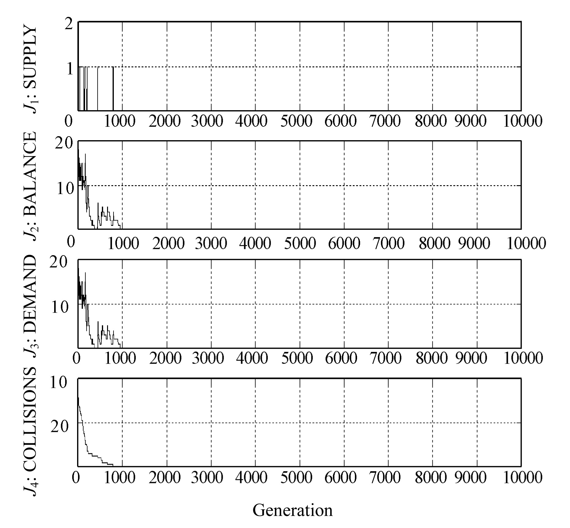
 The MOEA must obtain a set of solutions that satisfy the constraints of the problem, that is to say, possible solutions to the problem. Fig.6 shows the observed evolution of the algorithm until reaching these solutions.

Fig.7
Fragmentation and time optimization in MOEA

 In this figure we can see a response to the priority scheme shown in Fig.4. First of all the MOEA tries to minimize J₄ because its priority has been set to 1. Then the algorithm obtains possible solutions reducing to zero the value of J₂, J₃ and J₄. We can see fluctuation of these values due to their lower priorities with respect to J₄.

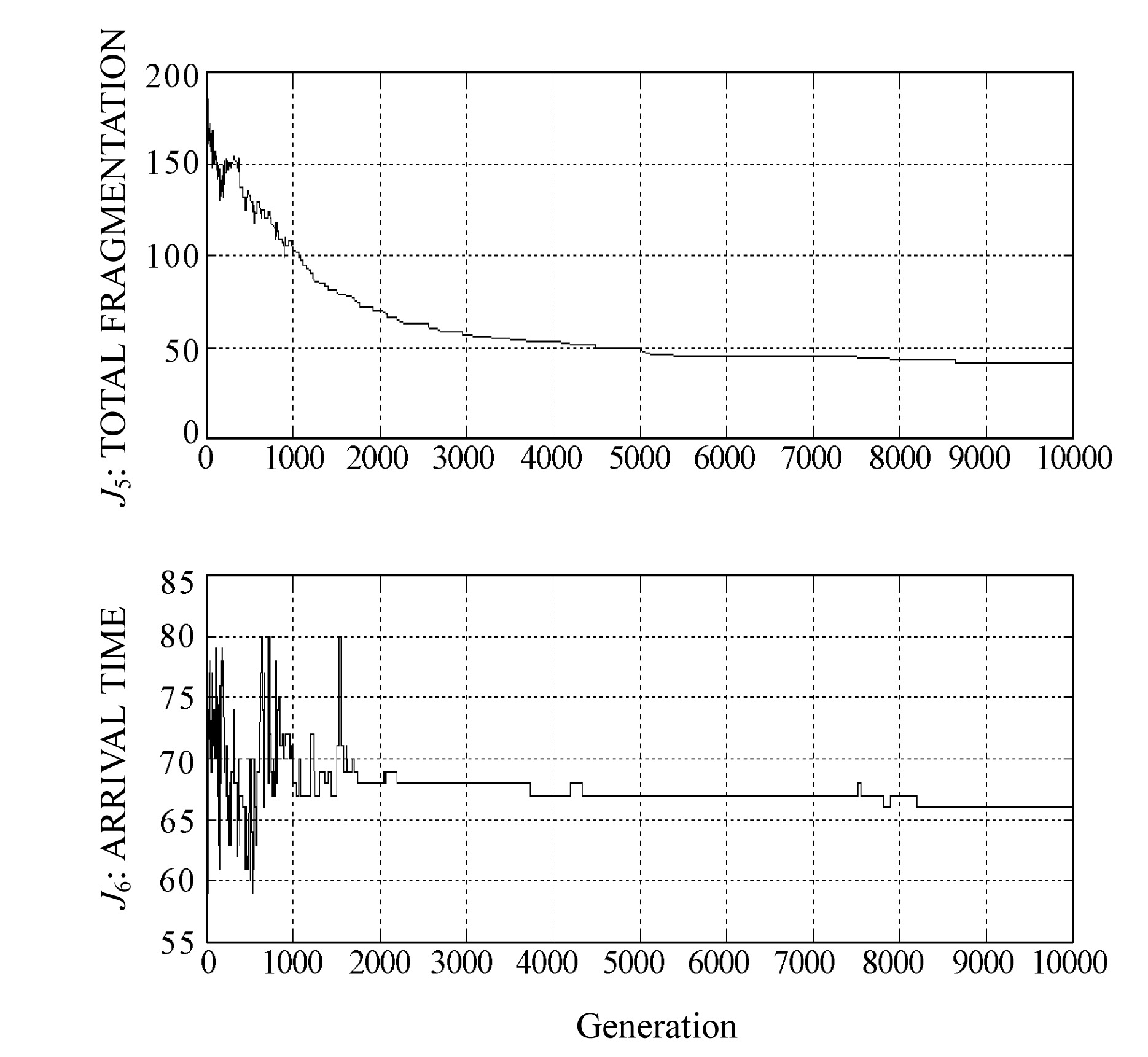
 Once there are possible solutions of the problem, the next objective is to minimize the fragmentation of the shipments. The number of groups of packages sent by each node appears in Fig.7. It is observed that they are reduced as the algorithm evolves. The arrival time stays within the established limits. In addition, whenever possible, this time is minimized.

Fig.8
Fragmentation obtained by MILP with T=66

 As the hard constraints are fulfilled after a few initial generations (over 1000 in this case) and J₅ is in the lower priority level, the MOEA searches for solutions which minimize the total number of packages first and so the evolution of this objective value monotonously decreases from generation 1000 to the end. As solutions with smaller number of packages are preferred to those with a lower total time, the evolution of J₆ is not always decreasing. While the number of packages is not decreased, the MOEA prefers those solutions with a minimal total arrival time, and as soon as a solution with a smaller number of packages is obtained by the algorithm that will be selected as the best of the current generation, no matter what happens with the total arrival time.

.  Results with MILP solver

 The MILP solver must obtain a set of solutions. Firstly the time has been optimized, looking for a reasonable value, T=66. If the time is set to 65, the solver iterations increase to twelve million, so the optimization process is aborted. We solved the problem with a PIII 500 MHz 128 MB RAM computer.

 Once the upper bound for the time is fixed, five solutions with ε=1 Eq.(22) are obtained. These solutions are given in Table 4.

Table 4

MILP solutions with T=66

Iterations	Fragmentation
0	160
1000	91
2000	49
3000	44
4000	43
5000	41

 The model had been solved using ILOG OPL (Van Hentenryck, 1999). ILOG OPL has the option to introduce in CPLEX searching a heuristic frequency set to 200. With this configuration the searching procedure is not in the same order in consecutive optimizations, so the number of iterations for each optimization is not increased. The representation is shown in Fig.8.

Fig.9
Flow diagram for the HYBRID algorithm

.  Results with hybrid algorithm

 Finally, we can use both solvers (MOEA and MILP) to implement a hybrid solver. To do that, we run both methods in parallel and use the solutions obtained by the MILP solver as immigrants for the MOEA. The MILP solutions are feasible solutions because these immigrants have J₁,…,J₄=0. Therefore we obtain an improvement in the convergence of the solutions obtained by the MOEA solver. Moreover the MOEA combines these solutions to improve the convergence of the MILP solutions too.

 The final algorithm implementing this feedback given by the MILP solutions is shown in Fig.9. The result is a hybrid algorithm that improves the convergence of both methods (MOEA and MILP) when used separately.

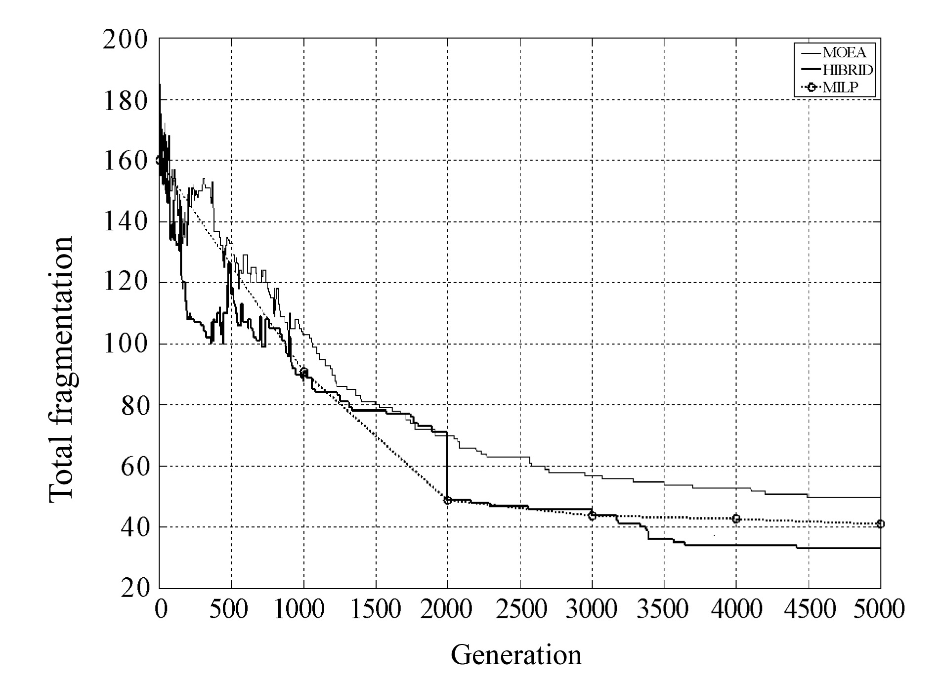
Fig.10
Fragmentation for the three methods

 As we can see, the algorithm consists of the periodical introduction of MILP solutions as immigrants in the MOEA population. In our case we introduce these solutions if the generation number is in the set of iterations shown in Table 4.

 If we run our network example for the three methods, the results obtained are shown in Fig.10.

 Here, we can see the evolution of the fragmentation among the three methods. The surrounding points represent the iterations in which the immigration of solutions takes place. The hybrid algorithm solutions are better in all the time. Then, the hybrid method improves feasible solutions more quickly than the MOEA or MILP.

.  CONCLUSION

 The optimization methods described in this paper provide an easy way for solving a combinatorial nonlinear optimization problem, namely the transport of products through a pipeline network.

 The developed algorithm uses the knowledge of the problem to let the MOEA converge at an acceptable speed. This knowledge is introduced while designing the coding of the problem solutions and uses a repairing operator that modifies the working strategies which do not verify part of the constraints imposed by the network.

 The implemented algorithm is flexible and can be used for different networks and problems specifications. While modelling the problems, several features are included in its definition to let the algorithm optimize a big range of networks. Any number of sources, intermediate nodes and destinies can be selected and bidirectional pipes are contemplated. Additionally, the types of products handled by each source can be different; the size and initial content of each storing tank for all the products, sources and intermediate nodes must be specified; and the correct time interval of products arrival in each destiny has to be defined.

 The MOEA and the MILP solver can avoid local optimal solutions and yield similar results. We have implemented a hybrid algorithm that gives better optimal solutions in a shorter time of execution.

References

[1] Bazaraa, M.S., Jarvis, J.J., Sherali, H.D., 1990. Linear Programming and Network Flows, Wiley, New York,:394-418. 

[2] Botros, K., Sennhauser, D., Jugowski, K., 2004. Multi-objective Optimization in Large Pipeline Networks using Genetic Algorithms. , Intenational Pipeline Conference, Calgary, Alberta, Canada, :

[3] Chankong, V., Haimes, Y.Y., 1983. Multiobjective Decision Making Theory and Methodology. , North Holland Series in System Science and Engineering, New York, :

[4] De la Cruz, J.M., Andrs-Toro, B., Herrn-Gonzlez, A., 2003. Multiobjective optimization of the transport in oil pipeline networks. , IEEE International Conference on Emerging Technologies and Factory Automation, 566-573. :566-573. 

[5] De la Cruz, J.M., Risco-Martn, J.L., Herrn-Gonzlez, A., 2004. Hybrid Heuristic and Mathematical Programming in Oil Pipelines Networks. , IEEE Congress on Evolutionary Computation, 1479-1486. :1479-1486. 

[6] Luenberger, D.G., 1984. Linear and Nonlinear Programming, 2nd Ed, Reading. Addison-Wesley, New York,:

[7] Marglin, S.A., 1967. Public Investment Criteria, MIT Press, Cambridge, MA,:

[8] Marriott, K., Stuckey, P.J., 1998. Programming with Constraints: An Introduction, MIT Press, Cambridge, MA,:

[9] Michalewicz, Z., 1995. Genetic Algorithms, Numerical Optimization, and Constraints. , Proceedings of the Sixth International Conference on Genetic Algorithms, Morgan Kaufmann Publishers, San Francisco, CA, 151-158. :151-158. 

[10] Schrijver, A., 1986. Theory of Linear and Integer Programming, Wiley, Chichester,:

[11] Van Hentenryck, P., 1999. The OPL Optimization Programming Language, MIT Press, Cambridge, Massachusetts,: