Similar articles

Abstract: The determination of initial equilibrium shapes is a common problem in research work and engineering applications related to membrane structures. Using a general structural analysis framework of the finite particle method (FPM), this paper presents the first application of the FPM and a recently-developed membrane model to the shape analysis of light weight membranes. The FPM is rooted in vector mechanics and physical viewpoints. It discretizes the analyzed domain into a group of particles linked by elements, and the motion of the free particles is directly described by Newton’s second law while the constrained ones follow the prescribed paths. An efficient physical modeling procedure of handling geometric nonlinearity has been developed to evaluate the particle interaction forces. To achieve the equilibrium shape as fast as possible, an integral-form, explicit time integration scheme has been proposed for solving the equation of motion. The equilibrium shape can be obtained naturally without nonlinear iterative correction and global stiffness matrix integration. Two classical curved surfaces of tension membranes produced under the uniform-stress condition are presented to verify the accuracy and efficiency of the proposed method.

一种用于薄膜结构形态分析的新型数值计算方法

研究目的：为轻质柔性薄膜结构初始形态的确定提供一种准确、高效的新型数值模拟方法。
创新要点：1.建立基于有限质点法（FPM）的柔性薄膜非线性计算理论，并将其首次应用于膜结构的形态问题分析之中；2.提出一种将动力控制方程通过积分转化为动量方程，并利用加速静力收敛策略，快速获得初始平衡状态的方法。
研究方法：1.基于向量式固体力学的基本概念，将分析域离散为一系列质点，建立有限质点法柔性膜结构计算模型，并用牛顿第二定律描述质点运动（图1~图3）；2.采用一套基于物理模式的分析步骤来描述分析对象的几何非线性变形，有效扣除刚体运动的影响以准确获得质点间的相互作用内力（图4~图7）；3.根据膜内给定的预应力分布，按照膜结构初始形态分析步骤进行循环迭代求解（图9）。
重要结论：利用本文算法确定膜结构初始形态，计算速度快、准确性高，并且求解过程中不会因非线性变形而引起数值计算方面的困难。

关键词：膜结构；有限质点法；形态分析；显式时间积分；初始平衡态

1.  Introduction

 Membrane structures have attracted considerable attention due to their light weight, high flexibility, and ease of stowing and deployment. The applications range from innovative architectural structures and space structures to medical appliances. A distinguishing feature of this type of structure is that it requires prestress to develop structural stiffness and to maintain a stable shape before any external load is applied. Therefore, for the structural function and strength satisfaction, a key step in the design of a membrane structure is to determine an initial configuration that respects the law of equilibrium for a feasible prestress distribution under given geometrical boundary conditions, especially for the gossamer space structures with high precision requirement of shapes (Jenkins, 2001).

 The topic of shape analysis has become an attractive research field since the pioneering work of Otto Frei in the 1960s and 1970s (Otto and Rasch, 1995). Early studies were conducted by direct physical modeling for visualization. A representative case was the soap-film analogy (Otto and Rasch, 1995; Lewis, 2003), which had the natural property of adjusting to a stable minimal surface with uniform stress in every direction. These physical methods can be tedious and inaccurate for a measurement of the geometry, and involve error magnification when measurements of the model have to be scaled up to a full-size structure. Thus, with the advent of the computer age, many researchers have paid attention to the numerical methods for handling this subject. The analysis methods can be normally categorized into three main families: the stiffness matrix methods, the geometric stiffness methods, and the dynamic equilibrium methods (Veenendaal and Block, 2012). As a typical example of the stiffness matrix method, the traditional finite element method (FEM) was described in (Haug and Powell, 1972; Argyris et al., 1974). It may have some limitations due to the high nonlinearity of membrane systems. Apart from its demand for extensive matrix manipulations, possible singularity of stiffness matrix and divergence may be encountered when the trial geometry is far from the equilibrium position. However, with some special treatments and modifications (Wüchner and Bletzinger, 2005), it still can be used to solve this problem effectively. As an alternative for finding feasible equilibrium shapes, the geometric stiffness methods can simplify the nonlinear analysis. It is represented by the force density method derived from special discretization and linearization techniques (Schek, 1974). Although this method enables fast determination of equilibrium surfaces, it should be pointed out that additional iterative procedures are inevitable when it is used to model minimal surface forms (Maurin and Motro, 1998; Pauletti and Pimenta, 2008), and thus some of its attractiveness is lost. Unlike the preceding two methods, in the dynamic equilibrium methods (e.g., dynamic relaxation method (DRM)), a steady equilibrium shape for an initially unbalanced structure is achieved by simulating a damped vibration process over time (Lewis and Lewis, 1996). Particularly, combined with the kinetic damping technique (i.e., resetting the nodal velocity to zero at each kinetic energy peak), this method has been presented as a powerful tool capable of finding forms of tension structures modeled by simple truss networks, linear triangular meshes (Barnes, 1999; Lewis, 2003) or high-order elements (Gosling and Lewis, 1996). Nevertheless, due to the introduction of many hypotheses for simplification (e.g., line elements and triple force elements) and the ignorance of shear deformation, both some errors and the tendency of meshes to distort may induce some inconvenience in the traditional dynamic relaxation-based methods (Wood, 2002).

 In recent years, some improved approaches based on the conventional techniques have also undergone significant development. For example, Brew and Lewis (2007) proposed an alternative methodology to the experimentally physical modeling on the basis of the free hanging concept. Moreover, using particle-spring systems, Kilian and Ochsendorf (2005) presented a novel approach for the exploration of funicular forms. This approach is also a kind of dynamic equilibrium method in nature. It is more suitable for treating the structural components with only axial deformation (e.g., cable or bar members), because for the solids, it is quite difficult to determine the spring stiffness that can represent the true material properties of the body exactly. Even if the body is discretized into equivalent networks, errors are still inevitable.

 In addition to the above techniques and approaches which have been extensively applied to shape analysis, the finite particle method (FPM) (Yu, 2010) that is derived from vector mechanics and superior in the complex structural behavior analysis (Ting et al., 2004), can be another choice for this subject. In FPM, the analyzed domain is regarded as a body composed of a finite number of particles, instead of a mathematically continuous body adopted in the traditional methods based on analytical mechanics. The motion path of each particle can be modeled via a set of discrete path units. Within each path unit, Newton’s second law, rather than weak variational formulations for the governing partial differential equations (PDEs), is adopted to directly formulate the motion of the particles. Interactions of a particle with its neighbors are determined by the elements connected with them. In the calculation procedure, an incremental theory based on the concept of the convected material frame (Shih et al., 2004) and an explicit time integration scheme for solving the equations of motion are also adopted. For further specific considerations, the FPM based on Ting et al. (2004)’s mechanics concept was developed, and was successively applied to the analysis of kinematically indeterminate bar assemblies (Yu and Luo, 2009a), deployable structures (Yu and Luo, 2009b), and progressive failure of truss structures (Yu et al., 2011).

 According to the analysis method classification aforementioned, the FPM belongs to the third category, i.e., the dynamic equilibrium methods. In FPM, neither the global material stiffness matrix nor the geometric stiffness matrix needs to be formed. In addition, there are some differences between the FPM and other dynamic equilibrium methods (e.g., DRM, particle-spring method), especially in the fundamental concepts and the procedure of interaction force evaluation. It should be noted that the FPM essentially employs a generalized mechanics frame which is capable of analyzing various complex behaviors. It is not a purely mathematical technique with introducing a fictitious mass and damping to the static equation to increase the numerical stability. Furthermore, in FPM, the convected material frames (i.e., the reference configuration) combined with other concepts, such as the path unit and the physical procedure of fictitious motion, are used to simplify the evaluation of interaction forces, while in some DR methods involving FE techniques, numerous matrix operations are required for calculating the finite rotation and deformation. Besides, the formulations of interaction forces in this method are rigidly derived from the theory of generalized large-deflection analysis of solids, instead of being a result of some simplifications (e.g., expressions in the form of element side/line forces or spring forces) as in some other DR methods. Therefore, a fine description of the internal force state can be obtained, even in some complex cases.

 In view of the remarkable performance of the FPM in tackling various nonlinear behaviors of structures, as well as its particular convenience for evaluating the prestress effect on tension structures, the primary purpose of this work is to extend the application of the FPM using a recently-developed 3-node triangular (T3) membrane element to the shape analysis of tension membranes. The remainder of the paper is laid out as follows. Section 2 provides a brief introduction of the fundamentals. Then, in Section 3, techniques for handling the geometrically nonlinear behavior of the T3 facet membrane elements are illustrated, and the formulations of interaction forces are derived. In Section 4, a solution procedure of shape analysis based on the FPM is developed, together with an improved time integration technique to reduce the computational effort. Section 5 presents two classical examples to verify the effectiveness of the proposed method in the shape analysis of stable minimal surfaces of tension membranes. Finally, some concluding remarks of this work are provided in Section 6.

2.  Fundamental theory of the FPM

 FPM is an intrinsic-modeling-based method designed to describe large rigid body motion and geometrical changes of a system of multiple continuous bodies. For simplicity, in this section, only a brief summary of the fundamental theory is provided by taking a 3D membrane as an example. More details can be found in (Ting et al., 2004; Yu, 2010; Yu et al., 2011).

2.1.  Point description

 Considering a continuous membrane as shown in Fig. 1, the motion of the membrane can be characterized by the trajectories of a finite number of discrete particles. Assume that the shape of a membrane undergoes a successive transformation from the initial configuration V ₀ to the reference configuration V_a , and then to the current configuration V. At the initial time t ₀, both the position x ₀ and velocity v ₀ of an arbitrary particle should be predefined. The subject to be addressed is converted to tracing the motion of each particle under the initial condition.




 An important concept in FPM is that particles are adopted as main variables to describe the parameters of a body, such as mass, geometry, and deformation, i.e., so-called point descriptions. At any moment every particle is in an eternal dynamic equilibrium state under resultant forces, whereas elements connecting particles to their neighbors do not carry any mass, and maintain static equilibrium during the motion. Hence, it ensures a strong form of energy balance for the entire system. Besides, particles are mutually independent, and thus all force calculations can be implemented in each element separately.

2.2.  Path unit description

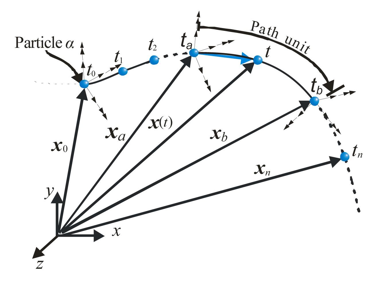
 Another characteristic of the FPM is the employment of a path unit. Referring to Fig. 2, it is assumed that an arbitrary particle α undergoes a motion during the analysis period, say from time instant t ₀ to t_n , with its position vector correspondingly changing from x ₀ to x _n . Such a trajectory can be split into n-discrete segments identified by a series of time points t ₀, t ₁, t ₂, t_a , t_b , …, t_n . Thus, the motion path of each particle within a segment, e.g., t_a ≤t≤t_b , is referred to as a path unit.




 Since the time interval is very small within each path unit, all variables (e.g., the constitutive law of materials, mass and topological relationships) can be regarded as constants with changes only at the boundary of a path unit, namely t_a or t_b . Consequently, the configuration of a deformable body at time t_a can be considered as the reference material frame for the evaluation of interaction forces.

2.3.  Governing equations of motion

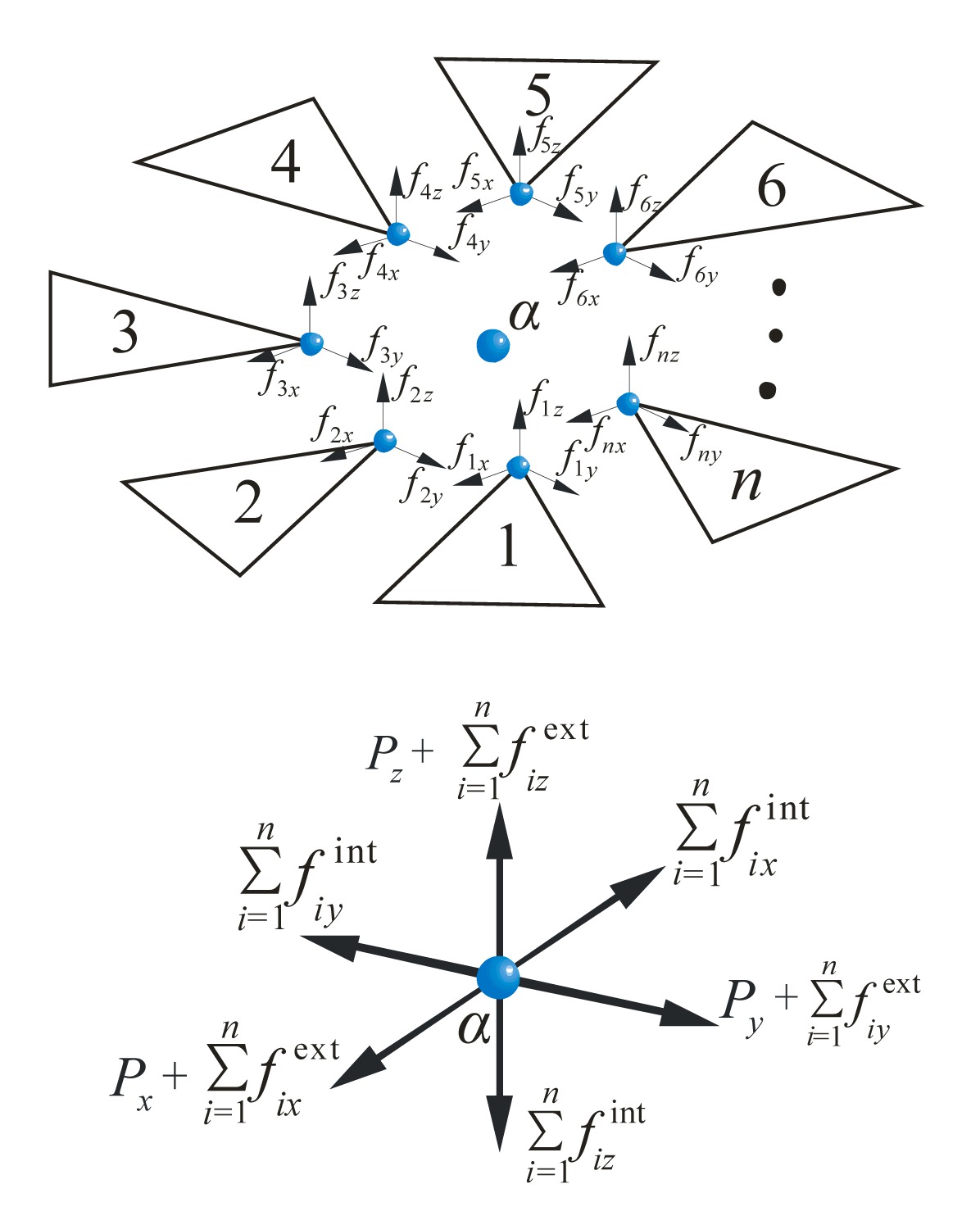
 As the foregoing assumptions in FPM, every particle is considered to be in a dynamic equilibrium state at any instant. Considering an arbitrary particle α, as illustrated in Fig. 3, its motion within each path unit is determined by the equation that follows Newton’s second law, that is (1) , where M _α is the particle mass matrix, represents the acceleration vector, and and denote the external force and internal force applied on the particle α, respectively.




 The determination of particle mass is a modeling procedure depending on an individual’s considerations for practical problems, rather than the results of some mathematic techniques. In this study, the mass term M _α is prescribed by the physical mass of the membrane, which can be defined as (2) , where m _α is the mass attached to the particle α, is the evenly distributed mass of the ith element jointing at the particle α, and n _c is the number of elements connected with the particle α.

  represents the internal forces of the particle α with its neighbors and it can be computed through an assembling procedure, that is (3) , where is the equivalent internal force contributed from the ith element connected with the particle α. The internal force evaluation is the most important work in FPM, which will be presented at length in Section 3.

  is the sum of the prescribed external forces acting on the particle α, that is (4) , where P _α is the concentrated force directly applied at the particle α, and is the equivalent force transformed from the distributed loads of the ith element according to the principle of virtual work.

2.4.  Description of kinematics

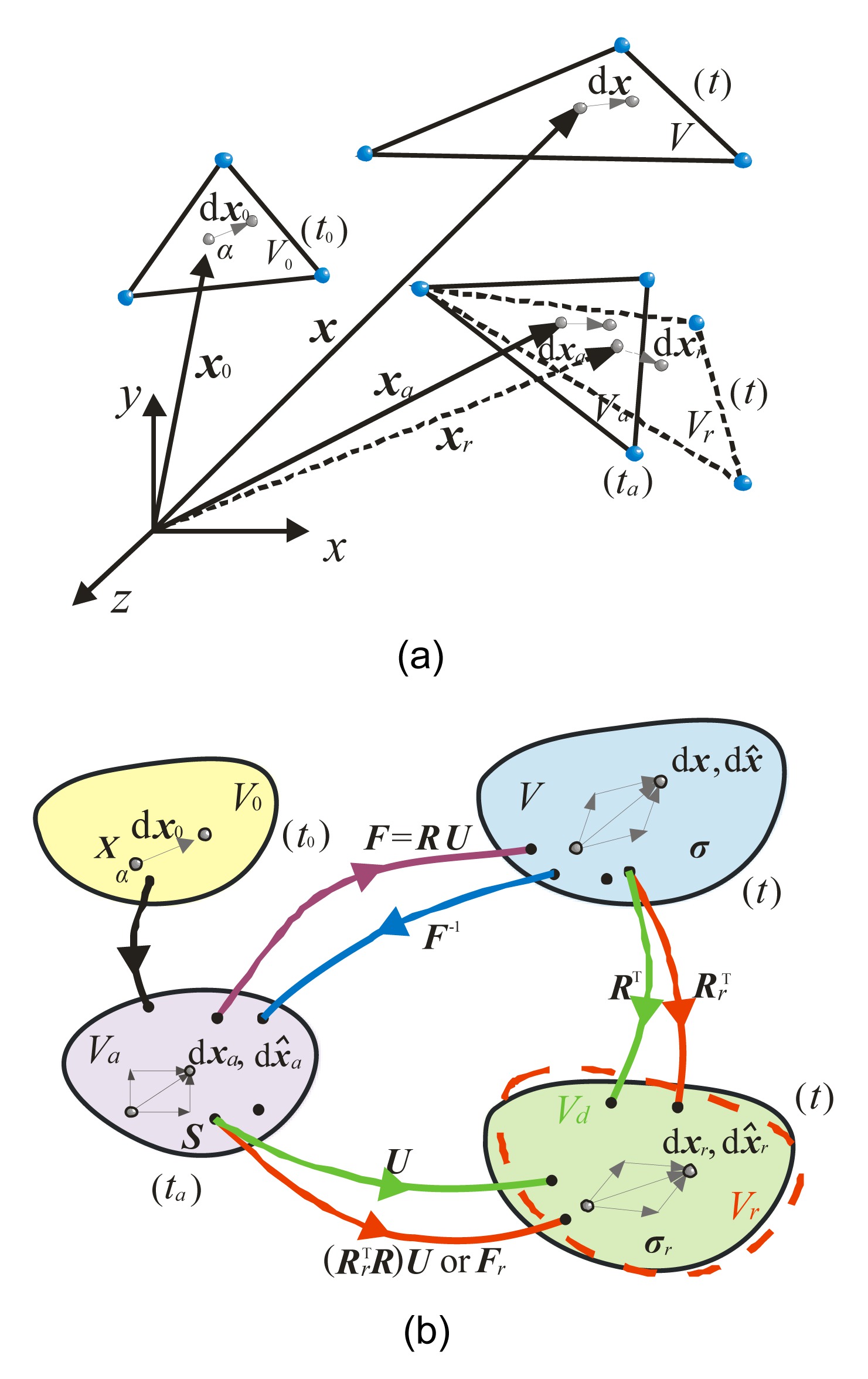
 According to continuum mechanics (Bonet and Wood, 1997), the deformation at an arbitrary point of a membrane can be described by the geometrical change of a differential element with an infinitesimal size. As illustrated in Fig. 4a, at time t_a the relative position vector of particle α to its neighborhood is denoted by d x _a . In FPM, the configuration at time t_a is taken as a convected material reference frame. After some time increments, at time t it changes to d x , that is (5) , where F is the deformation gradient due to the resultant forces. In terms of the polar decomposition theorem, the deformation gradient can be decomposed into the product of the rigid body rotation matrix R and the pure deformation gradient U . Thus, Eq. (5) can be rewritten as (6) .




 It is worth noting that R is only theoretically existent, because the rigid motion and deformation are fully coupled and it is rather difficult to get the exact deformation. In fact, only an approximation to the real one with the same order of magnitude as that of the residual rotation will be sufficient to obtain a convergent solution. Besides, there is an inherited predictor-corrector mechanism in FPM that prevents divergence even if the evaluation of the interaction forces is not absolutely accurate. Thus, in this contribution, a simple scheme for the measure of the average rigid body rotation is developed, which will be explained in detail in Section 3. Referring to Fig. 4b, let particles along with the element undergo a fictitious reverse rotation, and then the motion and deformation of the differential element can be expressed as (7) , where R _r represents an approximate average rotation, and F _r denotes the deformation gradient between V_a and V_r .

 As illustrated in Fig. 4b, V_d is a fictitious configuration after the reverse rotation with the accurate rotation matrix R ^T. The difference between V_d and V_r is merely a residual rotation, viz. , the order of which should be equal to or less than that of a pure deformation. Thus, it is not necessary to take into account the effect of the residual rotation on the calculation of strain. Moreover, for the convenience of defining independent degrees of freedom (DOFs), a set of deformation coordinates according to F _r are assumed. The corresponding strain, stress, and virtual work in the global coordinate system are (8) , (9) , (10) .

 With the transformation matrix Q that relates the global coordinates to the deformation coordinates at time t, Eqs. (8)–(10) can be rewritten in the deformation coordinate system as (11) , (12) , (13) .

 In addition, the relationship between the Cauchy stress and the second Piola-kirchhoff stress can be expressed as (14) . According to the principle of material frame indifference, the stress-strain expression should be formulated based on the pure deformation state. This requirement can be approximately satisfied when the strain, the stress and their relationships are defined at the fictitious state V_r which is very close to V_d , the exact state after pure deformation. Thus, if the geometric change is negligible as compared with the initial configuration at time t_a , the incremental strain can be simplified using the following infinitesimal strain (15) , where is the incremental deformation displacement vector. Given that and , a simple relationship for the incremental stress can be obtained from Eq. (14) (16) .

 From Eq. (16), it can be concluded that complicated stress updates for satisfying the principle of objectivity are not required, and the incremental stress can be defined as the engineering stress. Then, the total second Piola-Kirchhoff stress at time t, defined in compliance with the material reference frame, can be expressed in the deformation coordinate as (17) .

 The actual Cauchy stress at the current state can be obtained from the total second Piola-Kirchhoff stress through a pure rotation, that is (18) .

 Substituting Eqs. (15) and (17) into Eq. (10), the virtual strain energy at time t is (19) .

 In Eqs. (17) and (19), the Cauchy stress is a known quantity calculated by Eq. (18) in the previous path unit.

 Note that in FPM, the evaluation of the virtual work is only used for deriving the reaction forces acting on particles from each element, instead of solving the equivalent weak form of the PDEs of the entire system in terms of variational principles as in the FEM (Shih et al., 2004).

3.  Interaction forces in membrane structures

 In this section, a T3 facet membrane element is used to evaluate the interaction forces between particles within the membrane structures. Instead of adopting large strain tensors or simple coordinate transformations as in the common approaches, a physical modeling procedure is developed to handle the geometric nonlinearity.

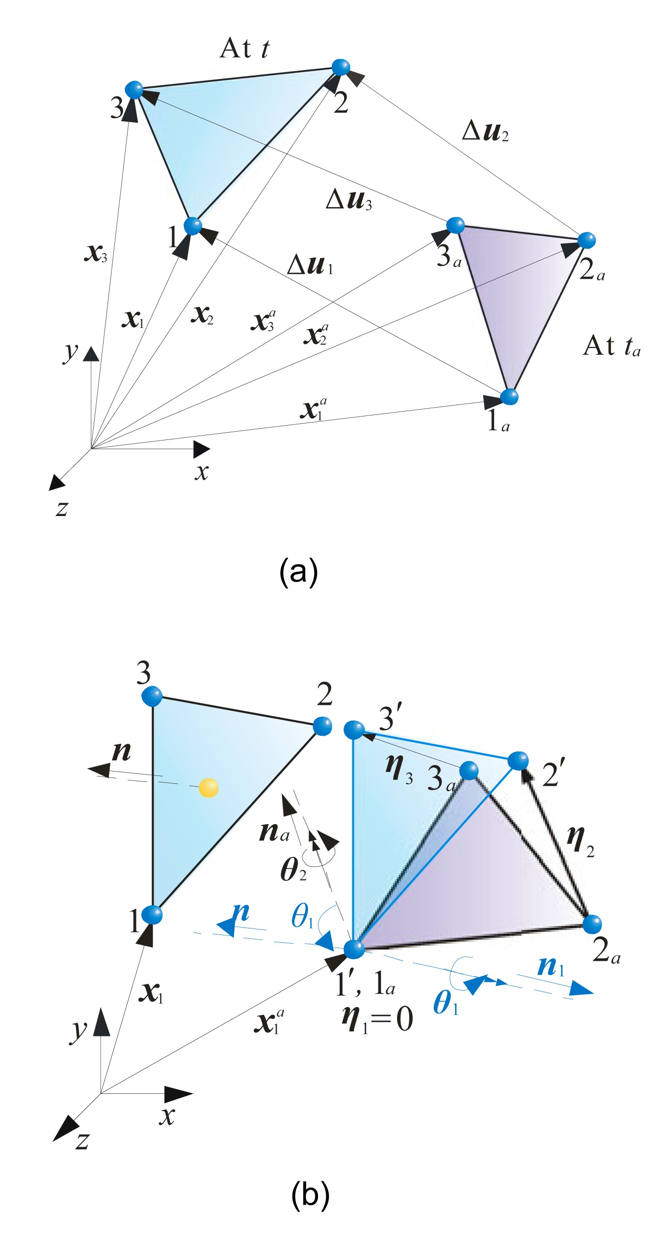
 For instance, consider an arbitrary T3 membrane element (1-2-3) with thickness h as shown in Fig. 5a, in which each node has three translational DOFs in the global coordinate system. Because the nodes of the element are rigidly connected with the particles, the position vectors of node i at times t_a and t can be defined as and x _i (i=1, 2, 3), respectively. Since the time interval between t_a and t is very small, both the material properties and the configuration are assumed to be unchanged within this time segment. If the configuration of the element at time t_a is chosen as the reference material frame, the displacement increment of node i between t_a and t is (20) .




 Note that the total nodal displacement increment Δ u _i includes pure deformation, rigid body translation, and rotation. For computational expediency, an efficient kinematical strategy is suggested here to extract deformation. As illustrated in Fig. 5b, it is assumed that the total rigid body rotation can be divided into two components, namely out-plane rotation θ ₁ and in-plane rotation θ ₂.

 Firstly, the angle of out-plane rotation can be conveniently measured by (21) , where n _a and n denote the normal vectors of a membrane element at time t_a and t, respectively. The corresponding rotation axial vector is (22) .

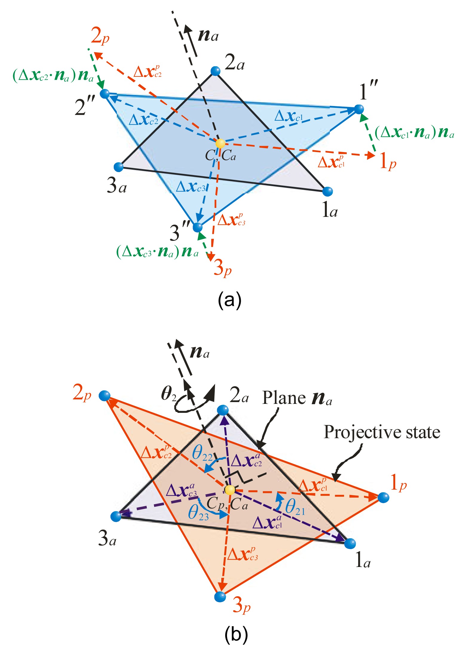
 Secondly, to account for the in-plane rotation, the element (1-2-3) is moved to make the centroids C_a and C coincide (C_a and C denote the centroids of the elements at time t_a and t, respectively), and then every node (1, 2, 3) of the element at time t is projected onto the plane (1 _p , 2 _p , 3 _p ) with normal vector n _a (Fig. 6a). Consequently, the projective nodes (1 _p , 2 _p , 3 _p ) and the element nodes (1 _a , 2 _a , 3 _a ) should be in a same plane. Then, the rotation angle with regard to node i can be evaluated according to the change of orientation for a line connecting node i with the centroid of the element, as shown in Fig. 6b, (23) , where and are the position vectors of node i with relative to the centroids of the element at time t_a and t, respectively, i.e., (24a) (24b)




 Then, the angle of in-plane rotation is approximately measured by the average of three node rotations, that is (25) .

 So far, the total rigid body rotation vector of the element (1-2-3) from t_a to t can be expressed as (26) , where θ is the angle of total rigid body rotation, and n _θ is the corresponding rotation axial vector, n _θ =[l m n]^T.

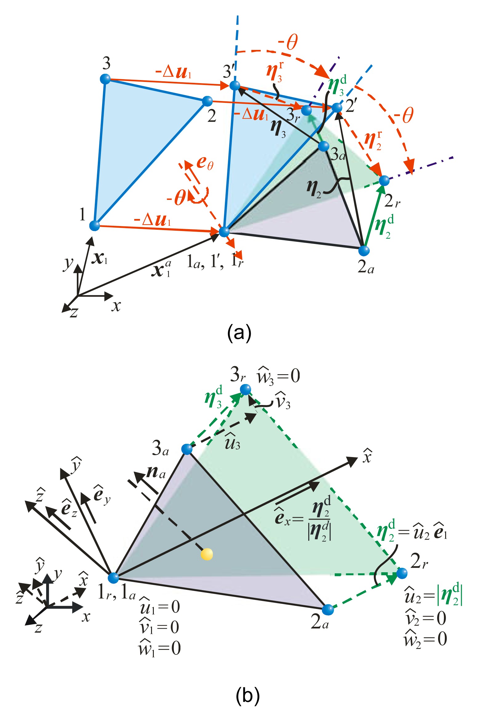
 Next, assume that the element (1-2-3) translates first with a fictitious reverse displacement (−Δ u ₁) to make the nodes 1 and 1′ coincide, and then undergoes a fictitious reverse rotation (− θ ) to arrive at the fictitious position V_r with the nodal labels changed to (1 _r -2 _r -3 _r ), as shown in Fig. 7a. When the fictitious reverse motion is completed, the pure deformation of the analyzed element can be obtained from a comparison of the configurations between the fictitious state V_r (1 _r -2 _r -3 _r ) and the reference state V_a (1 _a -2 _a -3 _a ). Therefore, the deformation displacement vector of node i from t_a to t is (27a) , (27b) , where η _i and are the total displacement increments of node i relative to node 1 and the rigid body displacement increment due to the fictitious reverse rotation of node i, respectively, and (28) , where R is a rotation matrix, I is a 3×3 identity matrix, and Ω ( n _θ ) is an angular velocity matrix expressed in terms of the components of the axial vector n _θ (Belytschko et al., 2000), .




 To evaluate the work equivalent internal forces acting on particles, a shape function with the same form as that developed in FEM is introduced for describing the strain distribution within the element. While different from the total displacements employed in FEM, the nodal variables here only account for the deformation. Therefore, the redundant DOFs corresponding to the rigid body modes must be eliminated to reduce the total independent variables to the correct number. To this end, a set of deformation coordinate systems are defined, with the origin locating at node 1 and the axis parallel to the deformation displacement vector of node 2, (also can be replaced by ), as shown in Fig. 7b. The basic vectors of , , and axes are denoted by , , and , respectively, that is (29) .

 Before the evaluation of the interaction forces can be implemented in the deformation coordinates, the deformation vector should be transformed to the new coordinate system first by (30) , where represents the coordinate transformation matrix from the global coordinates (x, y, z) to the local deformation coordinates .

 In the new coordinate system, six components (i.e., ) are zero, which implies that six DOFs are deleted. The remaining three non-zero deformation components are independent, and for convenience, they can be expressed in a condensed form, i.e., . Thus, the deformation displacements at an arbitrary point within the membrane element can be described by a set of linear interpolation functions similar to those in FEM, (31) , where is a condensed nodal deformation vector, and and are the shape function and the corresponding matrix form, respectively, where (i=2, 3), . With the deformation distribution functions, one can formulate the incremental strain and stress in terms of the elastic mechanics theory, and hence (32) , (33) , where denotes the constitutive matrix of the material under the plane stress condition referring to the stress state, and is the stress value at time t_a . If an isotropic elastic material is used, the matrix can be written as (34) . Then, substituting Eqs. (32) and (33) into Eq. (19), one can obtain the equivalent internal forces, (35) , where A_a and h_a denote the area and the thickness of the membrane element at time t_a , respectively.

 The other three components of nodal forces corresponds to the DOFs that have been eliminated in the deformation coordinate system, and thus they should be determined by the static equilibrium conditions of the element in the plane, namely (36a) , (36b) , (36c) .

 As a matter of fact, this equilibrium condition must be imposed to ensure that the internal virtual work remains unchanged even if subjected to a superposed rigid body motion, which is a requirement of the principle of objectivity for a continuum.

 Next, to assemble the equivalent interaction forces acting on a conjunct particle (i.e., summed by Eq. (3)), all the force components must be transformed to the global coordinate system. In addition, the element needs to undergo a forward motion, including a translation (+Δ u ₁) and a rotation (+ θ ), and to move back to the position at time t. Therefore, the actual internal forces at time t can be determined by (37) , where can be derived from Eqs. (35) and (36), R is a rotation matrix from Eq. (28) except that the rotation angle should be replaced by (+θ), and Q is a coordinate transformation matrix as that in Eq. (30).

 In the above formulations, magnitudes and directions of internal forces depend on the estimated rigid body rotation that may be not an exact value. A correction measure in displacements and rotations is thus generated in the subsequent calculation. In other words, if a particle moves too far from the equilibrium position due to the inaccurate evaluation in the previous step, the errors may exert effect on the calculation in the following step, which will increase the internal force in the opposite direction and pull the particle back to the equilibrium position. In short, the estimated rotation values, the equilibrium requirements of the elements and the equations of motion compose a self-predictor-corrector system in a natural way, which prevents the divergence due to the error accumulation.

4.  Computational procedure of shape analysis based on the FPM

4.1.  Solution strategy for governing equations

 Since every item in the governing equations of motion is explicitly expressed (Eqs. (1) to (4)), the structural response under given initial conditions may be explicitly obtained by replacing the nonlinear iterations with the recursions over time. Particularly, if a damping item is added to Eq. (1) to dissipate the kinetic energy of the system, the unbalanced force acting on each particle will be gradually reduced. In other words, every particle can naturally approach the equilibrium position and finally come to rest under the damping effect when the oscillations are progressively reduced. However, choosing a proper damping that is able to attenuate the pseudo-dynamic response in the shortest time is not easy. Moreover, in this study we mainly focus on the accuracy of the steady-state solution, while the transient process has no physical meaning and thus is not concerned. Therefore, to obtain fast convergence to the equilibrium shape, a modified integral-form time integration strategy is suggested here.

 Firstly, instead of directly solving the second-order force equation, we convert Eq. (1) into a first-order one (i.e., so-called a momentum equation of motion (Chang et al., 1998)) by integrating it with respect to time once, i.e., (38) , where and represent the time integral of the external force and the time integral of the internal force, namely the external momentum and the internal momentum, respectively. In the case of shape analysis, no external forces are applied, so .

 Then, assume that every particle satisfies a special condition similar to that of an initial value problem as follows: (39a) , (39b) , where and are used to denote the approximations to and , the theoretical integrals of the displacements from t ₀ to t_{n- 1} and from t ₀ to t_n , respectively. This condition implies that the displacement can be considered to be zero before time t_n , namely d _n =0 and d _{n −1}=0. Thus, the calculation of the integral function of the displacement at the following step, , is independent of the previous trajectory history. In the physical perspective, it suggests that the motion of the particles can be deemed to re-start from rest at each step. In this manner, the pseudo dynamic response of the discretized system can be effectively attenuated.

 It should be mentioned that the direct integration methods can be employed to computer the solutions of the new governing equation, and their basic properties in stability, accuracy, and convergence remain unchanged. If an explicit central difference formulation is adopted, an approximation to the velocity of an arbitrary particle α at time t_n can be given by (40) .

 Substituting Eqs. (39) and (40) into Eq. (38) and rearranging terms gives the time integral of displacement at time t_n explicitly, (41) .

 Then, the displacement of particle α at time t_{n+ 1} can be approximated in a finite difference form as (42) .

 In Eqs. (41) and (42), S is a positive parameter for accelerating the convergence procedure. The physical meaning of factor S is illustrated in Fig. 8. With the aid of this scale parameter, it can be expected that the rate of convergence will be improved. After a large number of trial calculations, it is also found that an empiric value of S on the order of 10² is appropriate when a similar rate of convergence can be obtained.




 The resulting formulation (Eq. (42)) seems similar to that of Euler’s method since they both employ the explicit difference format, but here we involve some special physical and mechanical considerations, rather than a pure mathematical technique for solving the differential equations of motion.

 It also can be found that the proposed time integration strategy only involves simple algebraic manipulations for vectors and at each step the solution may proceed particle by particle in a numerically uncoupled form. As a result, no global stiffness matrices need to be formed, and the requirement for the memory storage is very low.

4.2.  Procedure for initial stable shape analysis

 During the shape analysis implemented by the FPM, the calculation of equilibrium is always made based on a set of convected material frames, adopting a constant prescribed stress σ ₀ as the Cauchy stress (in Eq. (35)) at the beginning of each path unit. Moreover, we set the fictitious elastic modulus of the membrane model to be a very small value to ensure that the stress distribution in the equilibrium configuration is close enough to that of the specified prestress. However, the value of the modulus should not be zero, otherwise the self-error-correction mechanism (whereby the geometric change of an element can be suppressed by the interaction forces in the opposite direction induced by deformation) will become invalid, possibly leading to surface inaccuracy and irregular locations of particles that may be unusable for the subsequent load analysis in the design. After providing an appropriate initial arrangement of particles, we start the solution for the equilibrium shape of a membrane structure under given boundary conditions in which the displacements of the particles attached to the supporting systems are constrained. A recurrent calculation has to be carried out until the system reaches a steady equilibrium configuration according to the convergence criteria for the out-of-balance forces and the stress deviations, given by (43) , where the tolerances ε _F and ε _S are set to be very small values, so as to minimize the admissible influence of the dynamic response.

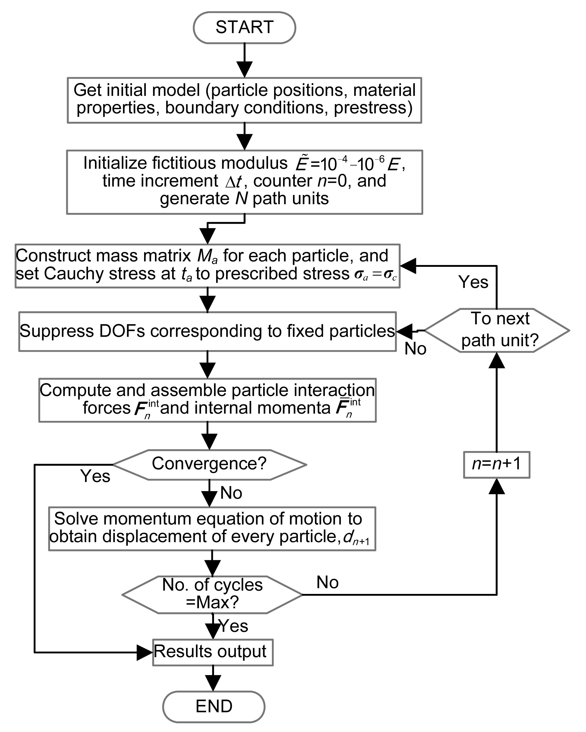
 The whole solution procedure outlined above for finding initial equilibrium shapes of tension membranes is summarized in the flowchart in Fig. 9. A self-designed C++ program has been developed to implement the proposed method that has been used for the numerical tests in Section 5.

5.  Examples

 To illustrate the performance of the proposed methodology, two well-known examples are described in this section: a catenoid and a Scherk-like surface. Both cases preserve the principle of uniform and isotropic tensile stress for driving the membrane towards an ideal equilibrium shape that minimizes the surface area under given boundary conditions, as observed in the soap film models (Lewis and Lewis, 1996; Wüchner and Bletzinger, 2005; Pauletti and Pimenta, 2008). The self-coded program for the numerical tests is run on a desktop PC with a CPU of Inter Core processor i5-2400 3.1 GHz and a memory of 4.00 GB RAM. All the results are obtained with the fixed tolerance values of ε _F=ε _S=10⁻³ for the convergence criteria.

5.1.  Catenoid

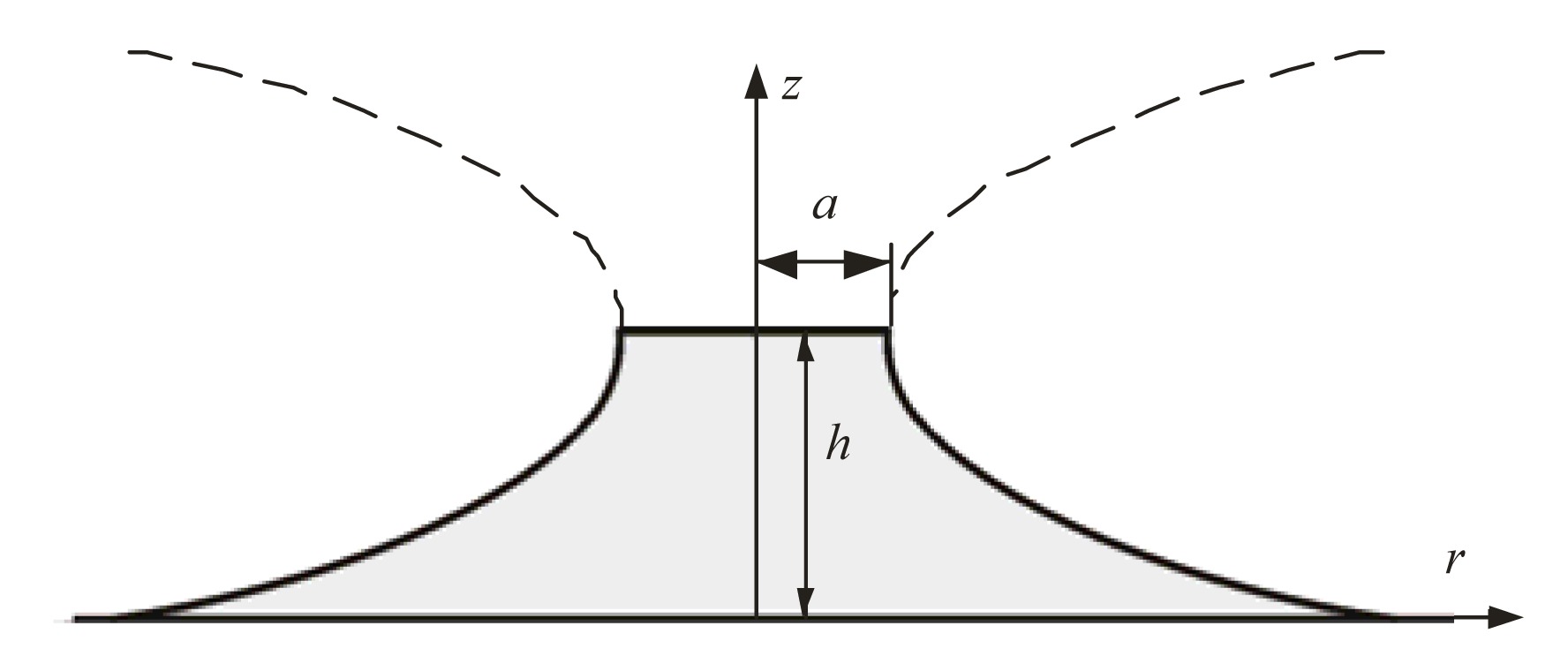
 The catenoid is the only minimal surface of rotational symmetry that can be described analytically, and thus it is commonly used as a benchmark shape-analysis case (Lewis and Lewis, 1996; Wood, 2002; Ye et al., 2011). The theoretical equation of a catenoid surface is given by (44) . In this example, a=12 m, h=27.5092 m are used and the sketch for the curvature shape of the catenary along the cross section is shown in Fig. 10.




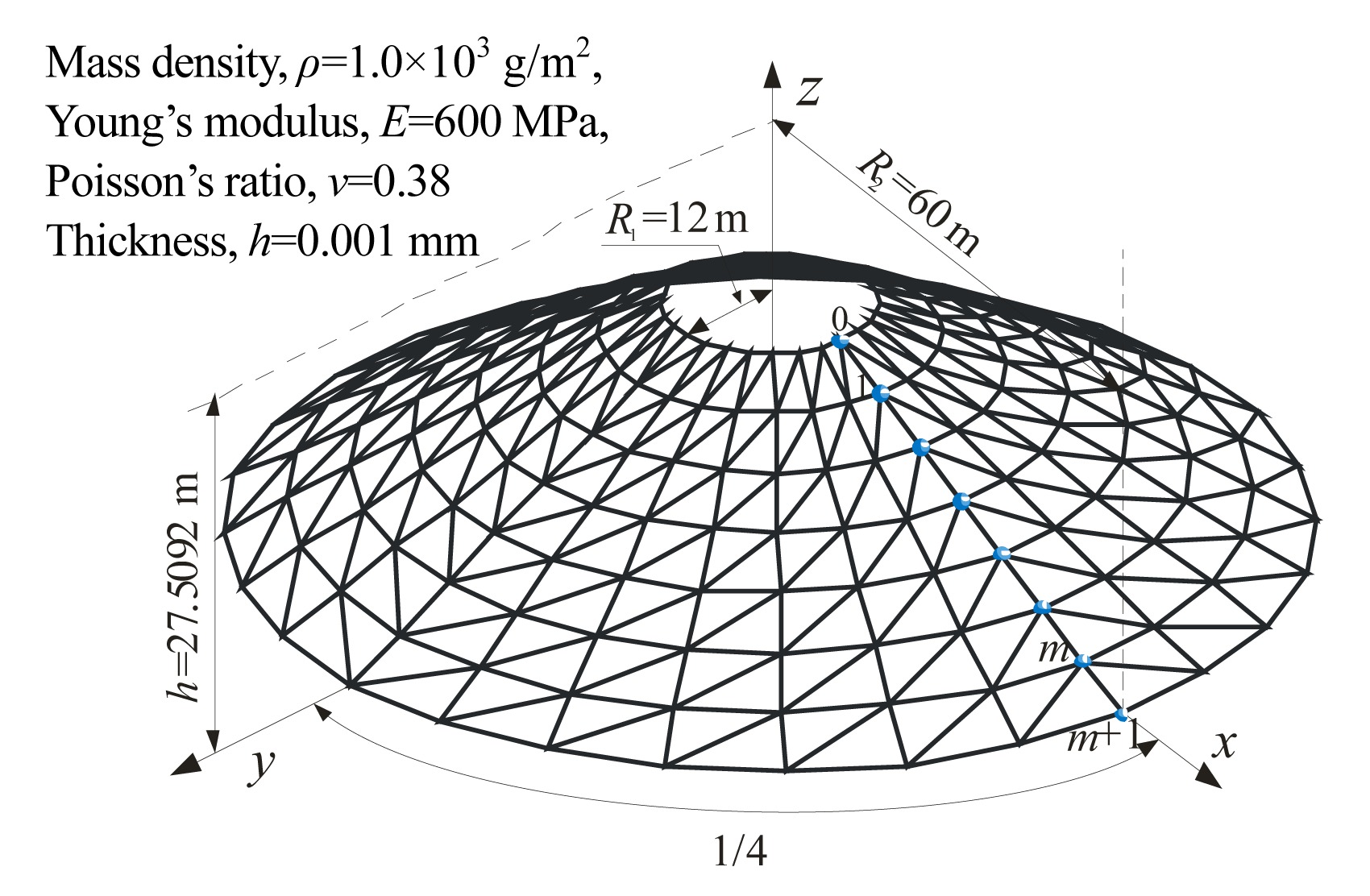
 The initial configuration of the analysis model is a conoid shape with fixed constraints imposed on the particles lying along the edges of two parallel rings with 12 and 60 m in radius and a distance of h apart to satisfy the boundary conditions determined by Eq. (44). Its geometrical and material properties are described in Fig. 11. A state of isotropic prestress, i.e., σ ₀=[σ_x σ_y τ_xy ]^T=[σ ₀ σ ₀ 0]^T with σ ₀=20 kN/m (force per unit width), is re-applied during the analysis process in order to obtain a close approximation to the minimal surface. Given the symmetric condition of the problem, only a quarter of the entire membrane is solved. To monitor the trend of convergence, three cases with different densities of particles (i.e., 49, 100, and 196 particles) are considered. An artificial scale factor S=100 for increasing the accumulative displacements, a time step Δt=10⁻⁴ s and a fictitious elastic modulus are employed for these numerical implementations. According to the given convergence criteria, the program respectively takes 182, 278, and 394 steps (corresponding to the three different models) to complete the solutions.




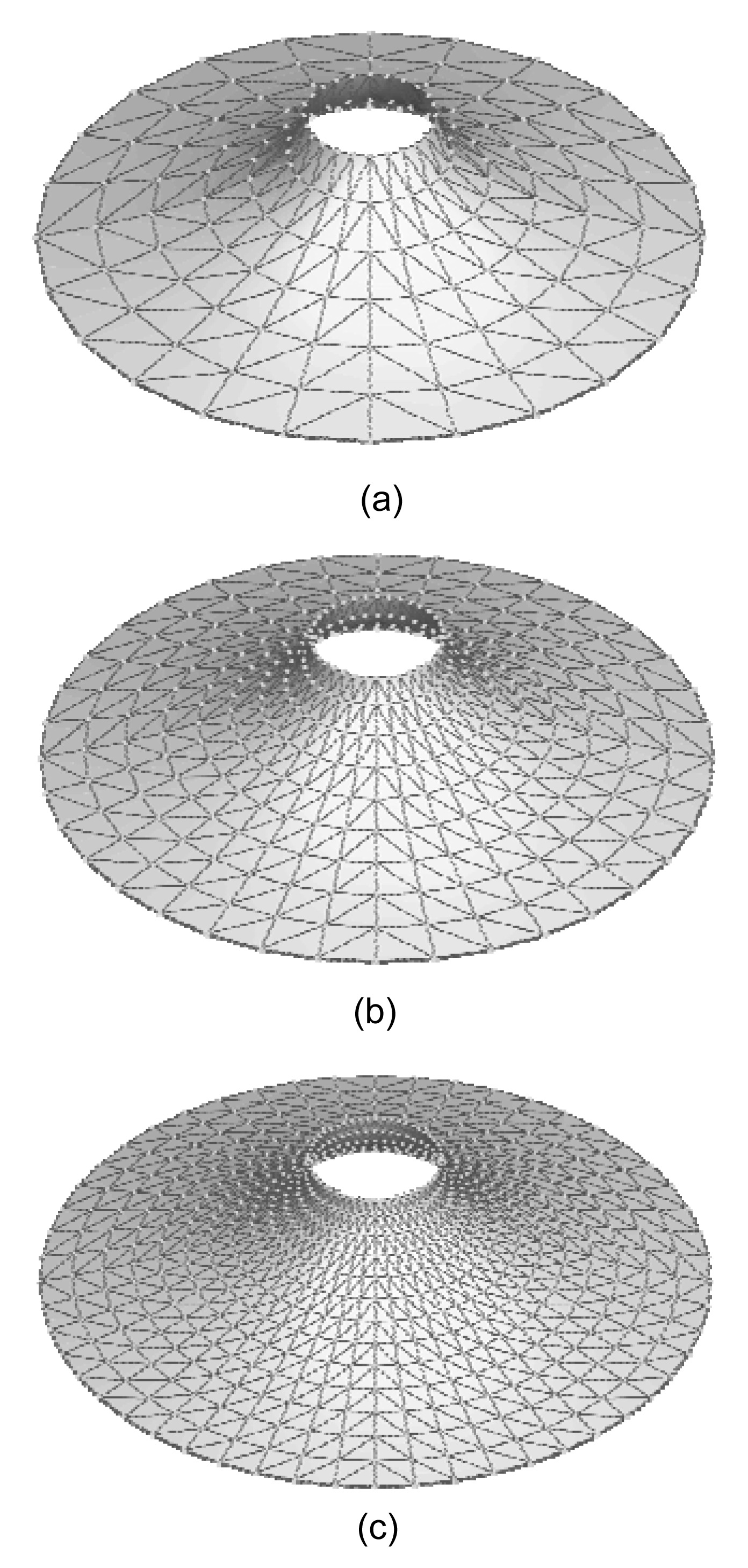
 Fig. 12 illustrates the stable-found shape of each model after analysis. It is noticed that all the particles are reasonably distributed across the final surfaces with regular spacing. The surface areas are 12 253.217 m², 12 186.362 m², and 12 149.755 m², respectively, giving errors within 1.5% of the theoretical value of 12 118.302 m². At the same time, the maximum root mean square (RMS) error (in the model composed of 49 particles) in the z-direction is only 0.431 m, i.e., 1.567 % of the height.




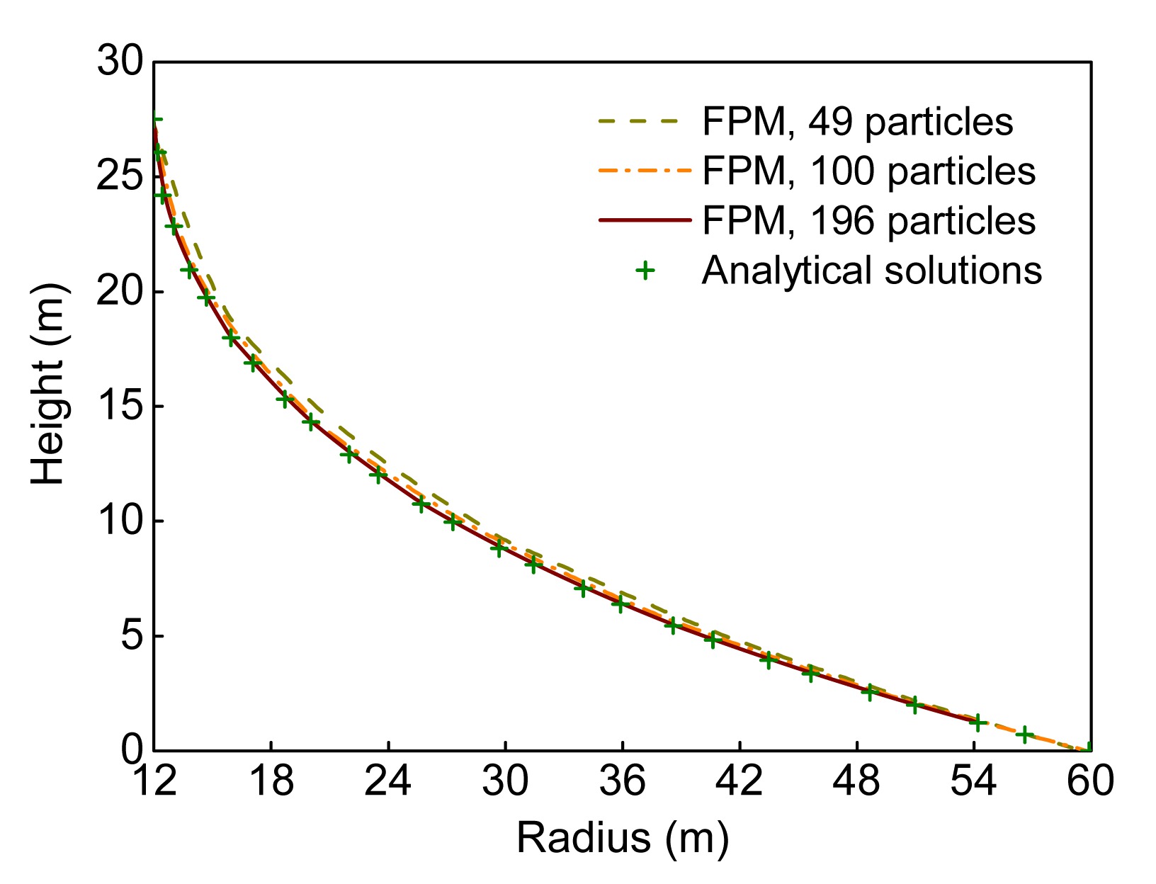
 The geometrical profiles of the sections of final surfaces across the diameter of the upper/lower ring are compared against the analytical solution in Fig. 13. It can be observed that the discrepancy is small even in the case of a coarse arrangement of particles, and the convergence trend is apparent as the surface discretization is refined.




 For comparison, DRM with kinetic damping (Lewis and Lewis, 1996) is also programmed and applied to this example. Note that the same level of discretization is employed by the DRM. The results of the comparative study on accuracy of FPM against DRM are displayed in Table 1, where the coordinates of the points marked with 1–m observed in Fig. 12 are presented and the errors are evaluated against the exact positions obtained from the theoretical equation. It can be found that both methods can provide accurate solutions. The results predicted by the FPM are a little closer to the theoretical values, though the improvement is very limited. However, the DRM has to monitor the kinetic energy of the entire system as the iterations proceed. Moreover, an extra effort for estimating the precise point of maximum kinetic energy and corresponding corrections for displacements are repeatedly required whenever an energy peak occurs. For the FPM, by contrast, it is not necessary to take into account any additional condition during the whole analysis process. Furthermore, with the aid of the fast integration strategy for static solutions, the FPM can handle the shape analysis of tension membrane structures more effectively, which will be further investigated in the next example.

5.2.  Scherk-like surface

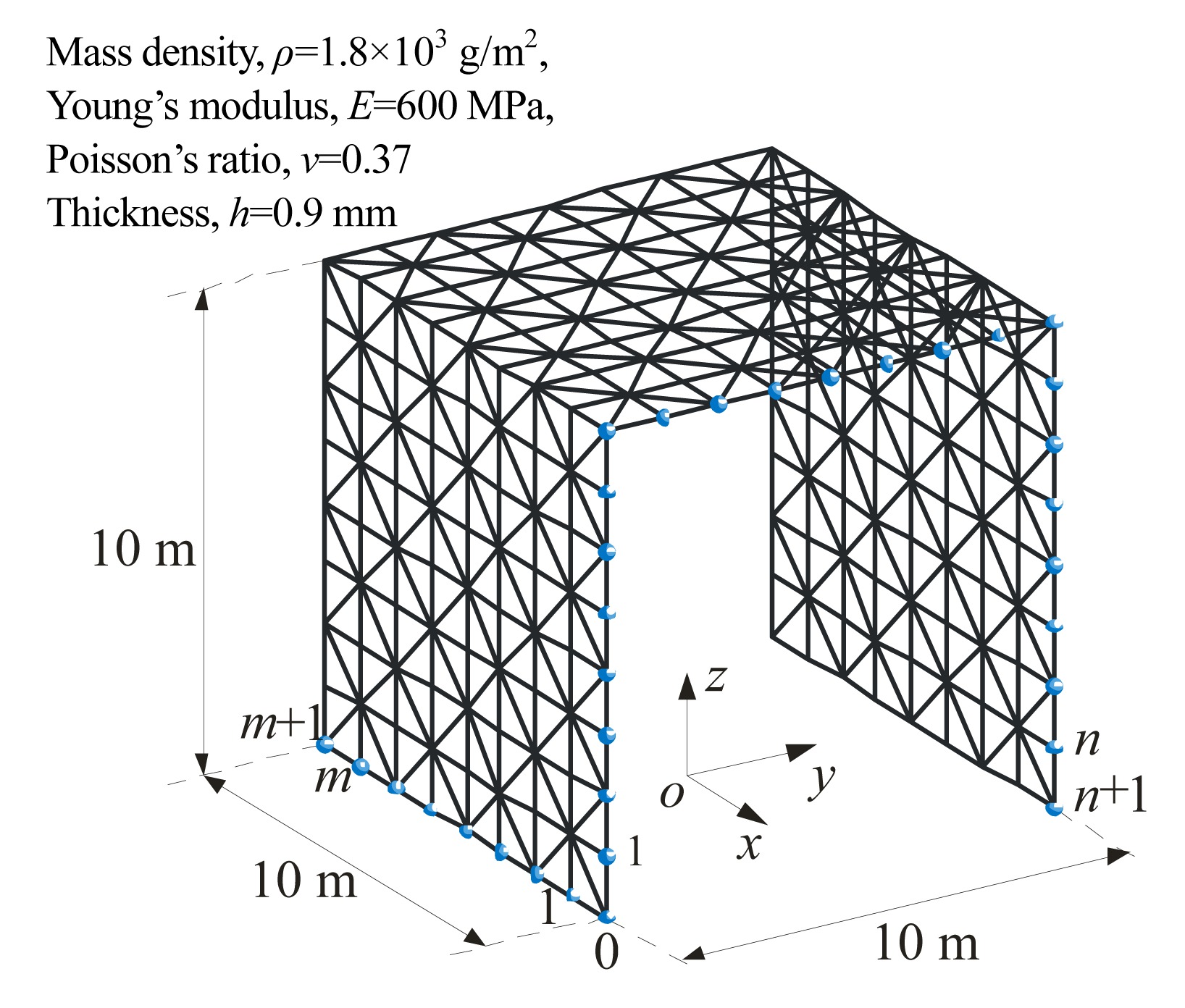
 Like the catenoid, the Scherk-like minimal surface (or referred to as a Box surface) is also a classic shape-analysis case, which has been previously studied by Maurin and Motro (1998), Brew and Lewis (2003), and Yuan et al. (2010). In this example, the initial configuration of the analysis model is a box shape which consists of three rectangular planes with the straight boundaries following the edges of a cube. The geometrical and material properties of the box model are specified in Fig. 14. To achieve the stable minimal surface, an isotropic and uniform prestress with σ ₀=20 kN/m and a scale factor S=100 are also employed. The fictitious elastic modulus is set as and the size of time step is Δt=5×10⁻⁴ s.




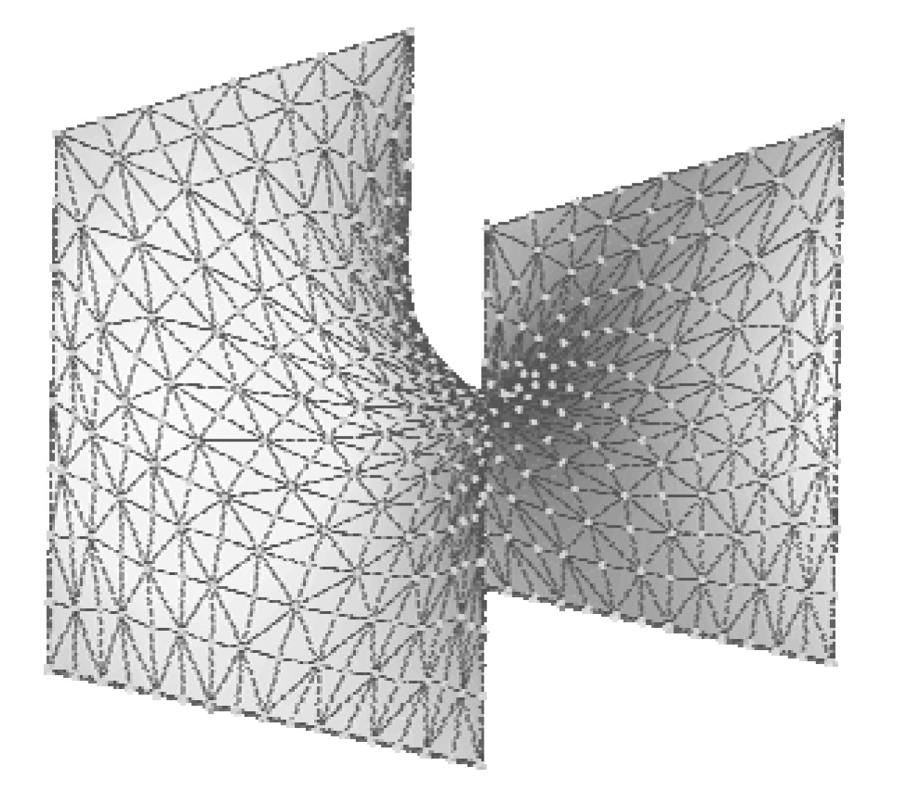
 In the case of a dense arrangement of particles (425 particles), the final equilibrium surface spanning the rigid boundary frame is represented in Fig. 15. The final area of this surface is 246.28 m², which shows good coincidence with the exact geometry, as that obtained by Yuan et al. (2010).




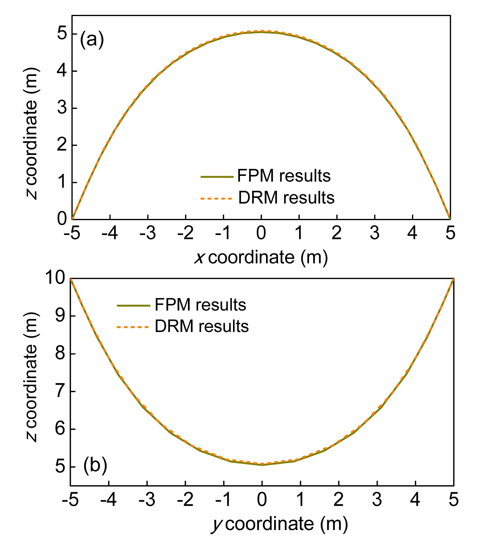
 Here, since the theoretical solution is not known, the results generated by DRM based on Barnes’s formulations (Barnes, 1999) are used for the assessment of accuracy. Figs. 16a and 16b show the profiles of the sections of the surfaces across the x-z and y-z central planes, respectively. A visual comparison shows that the discrepancy between the results predicted by FPM and those generated by DRM is not apparent. It also can be found that the center point at the top of the profiles lies very closely to midway between the top and bottom boundaries, with a slight deviation of only 0.536% of the height range, as necessitated by the zero mean curvature required for the minimal surface and the symmetry of the boundaries as well.




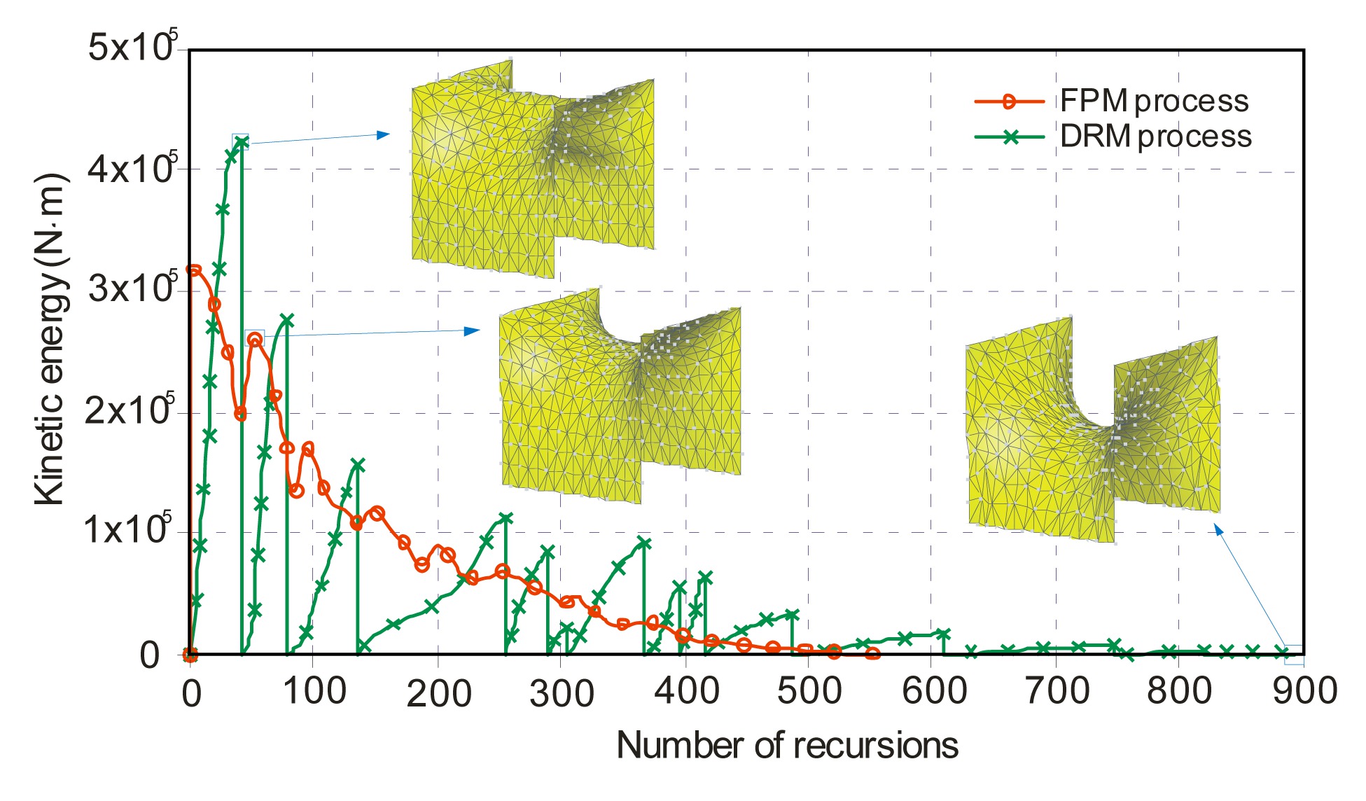
 For a better investigation of the solution process, the variations of kinetic energy (KE) of the entire system with the iteration history and the shapes of the membrane structure at different steps are plotted in Fig. 17. As predicted, the KE becomes smaller and eventually approaches zero, as more computation steps are taken in the implementations of both methods. In details, it is noticed that the decrease trends of KE during the solution process are almost the same for both methods, but with the FPM, a much smoother convergence process for attenuating the pseudo-dynamic oscillations can be achieved within a shorter iteration history, when compared with the DRM with kinetic damping.




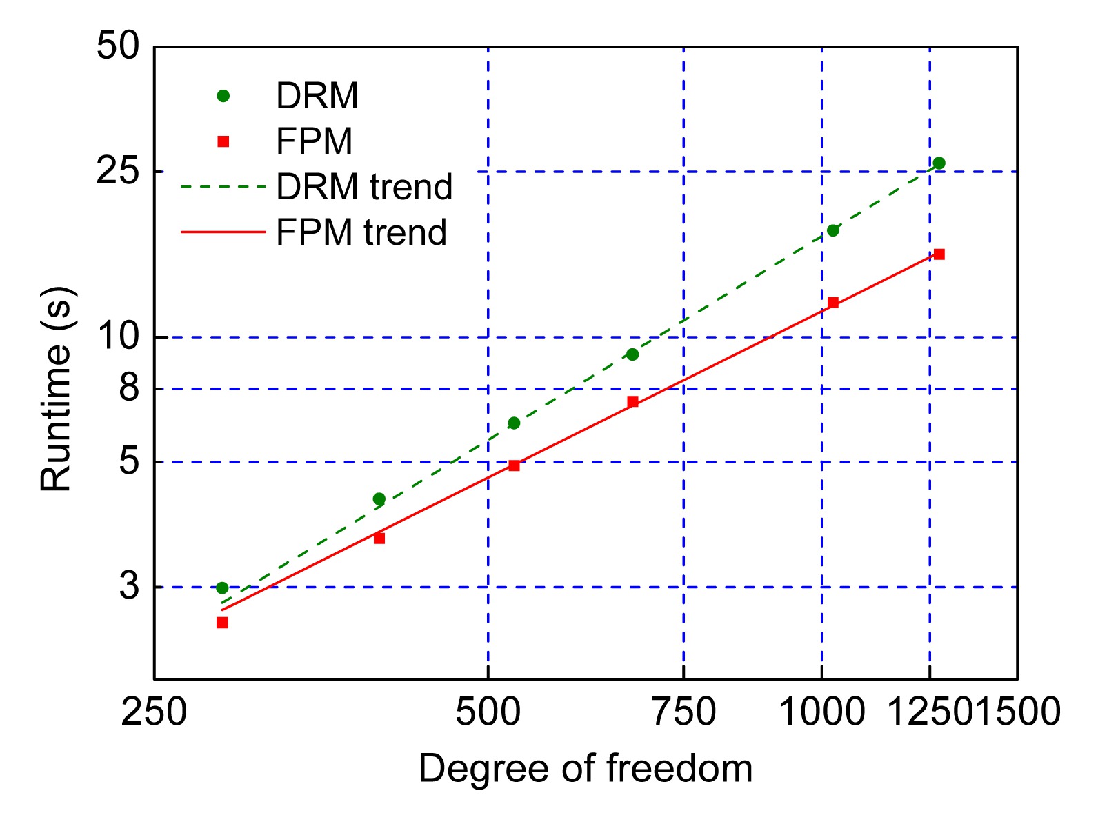
 Table 2 gives the results concerning the relative efficiency of the two methods for increasing DOFs, in terms of the number of iterations for convergence, the amount of time per iteration, and the total runtime required by FPM and DRM, respectively. One can observe that the slightly more computational effort of the FPM per step can be compensated well by the fairly decreased number of iterations for completing the solutions. Obviously, the FPM using the proposed formulations combined with the fast time integration strategy exhibits a higher convergence rate, so that a maximum reduction of solution time up to around 40% has occurred while a result of equal accuracy still can be achieved as compared to the DRM. Based on these results, it can be reasonably deduced that the FPM has a potential for an efficient analysis of large and complex structures with sufficiently fine discretization for ensuring accuracy. This statement is also documented in a comparison of the performance between the two methods as shown in Fig. 18, where the relationship between the influence of the level of discretization input and the time taken for the calculation to terminate is further illustrated. This comparison reveals that the time cost increases approximately log-linearly with the DOFs for both methods, but at a little lower rate for the FPM. To sum up, the proposed method can mimic the solutions generated by the DRM very well while considerably reducing the computational costs, especially when the size of the problem is enormous.

6.  Conclusions

 This study presents a general FPM framework for investigating the shape analysis of tension membrane structures under given boundary conditions. An efficient numerical procedure of generating viable initial equilibrium shapes is given. If this method is applied iteratively with constant and isotropic stress prescribed at any given point on the surface, it can lead to a stable minimal surface. The analysis of two classical tension membranes characterized by minimal surfaces has been conducted using a program following the proposed formulations and solution strategies.

 In FPM, the rigid body motion can be simply decomposed from the total displacement increments by fictitious reverse motion without complicated and time-consuming matrix operations, which makes it convenient to deal with nonlinear problems. At the same time, the modified explicit time integration strategy which is expressed in the form of momentums in place of forces, can efficiently reduce the computational effort in search of a steady equilibrium shape. Besides, during the entire analysis, no global stiffness matrices need to assembled or solved, and no iterations to follow nonlinear laws are necessary as well. Moreover, the effect of prestress can be readily exerted on the particles, and the final equilibrium shape can be naturally obtained as the limit of the pseudo oscillations without introducing any special treatment or modification to cope with the common numerical instabilities. Thus, it has inherent advantages in the shape analysis of tension membranes.

 From the numerical examples, the ability of the proposed method to obtain the accurate minimal surfaces of tension membrane structures has been verified by the comparisons with the analytical solutions and the numerical solutions of the DRM. It also has been proved that the FPM is much more efficient, in terms of the total CPU time required for convergence, than the DRM. In addition, no significant mesh distortion that may lead to poor representation of a surface occurs in this study. All these facts indicate a great promise for developing FPM into a general and effective method for shape analysis and further shape optimization of large-scale complex tensile structure systems that have potential applications in civil and aerospace engineering.

Acknowledgements

The authors would like to express their gratitude to Prof. Edward TING of Purdue University, USA for his advice and encouragement during the preparation of this work.

---

* Project supported by the National Natural Science Foundation of China (Nos. 51025858 and 51178415)