Wu-jun Chen, Jin-yu Zhou, Jun-zhao Zhao. Computational methods for the zero-stress state and the pre-stress state of tensile cable-net structures[J]. Journal of Zhejiang University Science A, 2014, 15(10): 813-828.
@article{title="Computational methods for the zero-stress state and the pre-stress state of tensile cable-net structures", author="Wu-jun Chen, Jin-yu Zhou, Jun-zhao Zhao", journal="Journal of Zhejiang University Science A", volume="15", number="10", pages="813-828", year="2014", publisher="Zhejiang University Press & Springer", doi="10.1631/jzus.A1400080" }
%0 Journal Article %T Computational methods for the zero-stress state and the pre-stress state of tensile cable-net structures %A Wu-jun Chen %A Jin-yu Zhou %A Jun-zhao Zhao %J Journal of Zhejiang University SCIENCE A %V 15 %N 10 %P 813-828 %@ 1673-565X %D 2014 %I Zhejiang University Press & Springer %DOI 10.1631/jzus.A1400080
TY - JOUR T1 - Computational methods for the zero-stress state and the pre-stress state of tensile cable-net structures A1 - Wu-jun Chen A1 - Jin-yu Zhou A1 - Jun-zhao Zhao J0 - Journal of Zhejiang University Science A VL - 15 IS - 10 SP - 813 EP - 828 %@ 1673-565X Y1 - 2014 PB - Zhejiang University Press & Springer ER - DOI - 10.1631/jzus.A1400080
Abstract: This paper proposes an extended design concept and mechanical description for cable-net structures, including 10 states and 15 procedures which are defined according to their physical nature and analytical capabilities. In the pre-stress release analysis, an iterative computational method is developed for the inverse evaluation from the equilibrium state to the zero-stress state, which adopts the least norm least square approach (LNLS) to the compatibility equation because of the indeterminate property of a cable-net structure. In the pre-tensioning development analysis, another iterative computational method is developed for the positive problem from the zero-stress state to the actual pre-stress state by moving the boundary joints, in which the explicit governing equations are formulated based on the particular energy function and a feasible self-stress mode is adopted to avoid the singularity of the initial stiffness matrix. To implement these methods, Matlab algorithms are developed and two examples are investigated. By comparing the results of the iterative method with those of the dynamic relaxation method, this study determines that they are comparable with each other, which validates the efficiency and accuracy of these iterative methods.
Darkslateblue:Affiliate; Royal Blue:Author; Turquoise:Article
Article Content
1. Introduction
Cable-net structures have attracted considerable interest from architects due to their lightweight, innovative forms, and environment-friendly characteristics. Despite the advantages of cable material, such as high strength, high modulus, and low relaxation, cable-net structures cannot be stable without having enough pre-stress state which forms a specific shape for structures and develops stiffness to carry loads. Consequently, the structural performance and the design process become rather complex, which provides great challenges to structural engineers.
As many analytical methods have been proposed, the common design process for cable-net structures consists of two basic steps. The first step is a form finding process to determinate the equilibrium configuration of a prescribed pre-stress state within a certain boundary, in which no material parameter is needed, as the required form depends only on the pre-stress state. The second step is a static and dynamic analysis under various load conditions (pre-stress, self-weight, snow, wind, and so on), in which material parameters are assigned to structures.
In the first step, extensive form finding methods have been developed, including those based on the dynamic relaxation method (Day and Bunce, 1970; Lewis et al., 1984; Barnes, 1994), the modified Newton-Raphson iteration (Argyris and Scharpf, 1972; Argyris et al., 1974; Haber and Abel, 1982), the force density method derived from special linearization techniques (Schek, 1974; Linkwitz and Grutndig, 1987; Gründig et al., 2000), the new adaptive force density method for particular tensegrity, and the updated reference strategy for membrane and cable structures (Bletzinger and Ramm, 1999; Bletzinger et al., 2010). In the second step, starting with the pre-stress analysis, loading analyses are carried out in sequence. To explore the structural behavior with respect to various load conditions, many researchers studied the resistant capacity of cable nets (Castro-Fresno et al., 2008; Del Coz Diaz et al., 2009) and the slope stabilization of flexible systems (Blanco-Fernandez et al., 2011; 2013).
Furthermore, the above two steps are assumed to be decoupled and carried out separately in the common design process; however, this assumption is applicable only if the differences between the final stress and the required stress are relatively small and negligible. The achievement of the required stress and shape has been investigated in extensive research. Argyris et al. (1974) found that the final stress was even 30% smaller than the required stress in an experiment performed on the Munich Olympic Stadium cable-net roof. Chen and Zhang (2008) discovered large stress differences in the suspended cable net of the 2008 Beijing Olympic Games and the central sail cable-net roof of the China Maritime Museum. Furthermore, Chen and Zhang (2011) also found that the final stress was even 16% smaller than the required stress in a 73.2 m span hyper cable-net roof. It appears that for a cable-net structure, the effect of the pre-stress discrepancy on the overall structural behavior is fairly enormous, which means the aforementioned assumptions are actually invalid.
To evaluate pre-stress discrepancies and describe their mechanical behavior, Wagner (2005) provided an enhanced design process for tension structures. Chen and Zhang (2008) and Zhao et al. (2012) also proposed an extended framework for the cable design process and developed an approximation method to minimize and eventually eliminate these discrepancies. Furthermore, Eriksson and Tibert (2006) proposed a routine for the pre-stress optimization of an offset tension truss antenna to reduce discrepancies. However, although many studies targeted the elimination of pre-stress discrepancies, substantial progress has not been completely achieved and there is still a need to extend the design process and clarify more clearly the mechanical behavior. Furthermore, it is also necessary that the design process should be standardized by modular procedures which can be carried out individually.
Firstly, this paper proposes an extended concept for the cable design process based on our previous study. The corresponding flow chart, which allows a highly detailed description of the stress state and simulation procedure, is added to clarify the mechanical behavior. Sequentially, iterative computational methods for the theoretical zero-stress state and the “actual” pre-stress state are developed to implement the extended design concept. In addition, Matlab algorithms are developed accordingly and two examples are proposed to demonstrate the efficiency and accuracy of the algorithms. For simplicity, the main assumptions throughout this paper are as follows: the analyzed cable-net structure is always under the linear-elastic scope with a small strain and large deformation; and it is simplified to be a pin-jointed link assembly whose cable link is straight with a uniform cross-section.
2. Extended design process and mechanical description of cable-net structures
For mechanical detailed modeling of a cable-net structure, it is essential to provide a correct mechanical description of its state and deformation process because of the arbitrarily large displacement which occurs in the loading state and in the building process. This study starts with a description of individual configurations throughout the entire life span of cable-net structures, before investigating the governing equations for each design step.
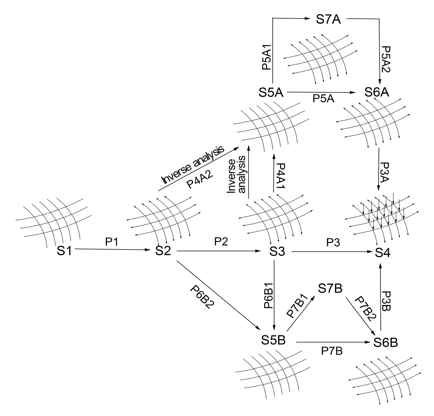
As shown in Fig. 1, a new extended design concept is proposed based on our previous work (Chen and Zhang, 2008; 2011), including 10 states labeled S and 15 procedures labeled P, which are defined according to the physical nature and analytical sense of cable-net structures.
Fig.1 Extended design concept of cable-net structures
The specific definition of every state is as follows: S1 defines the prescribed stress, boundary conditions, geometry, and topology; S2 is the equilibrium state, i.e., the resulting shape of the form finding; S3 is the pre-stress state of the common tensile structural analysis; S4 is the loading state (e.g., snow, wind, and so on); S5A and S5B are two assumed zero-stress states for assembled cables without gravity and pretension, and S5B corresponds to the real state where the entire cable-link assembly has been assembled together with connector clamps and lying on the building site; S6A is a theoretically predicted construction state, i.e., “actual” pre-stress state, whereas S6B is the final construction pre-stress state in reality; S7A and S7B are the intermediate states from the zero-stress state to the pre-stress state.
Accordingly, 15 procedures are designed to analyze the transformation from state to state. P1 represents the form finding analysis, and P2 represents the pre-stress analysis with the assignment of a material parameter and pre-stress on the equilibrium configuration of the form finding. Furthermore, P3, P3A, and P3B represent the loading analyses under various loads. In contrast to the common design process which merely includes the procedures from P1 to P3, the extended design concept also includes: P4A1 and P4A2 which represent the pre-stress release analyses; P5A, P5A1, and P5A2 which represent the pre-tensioning development analyses from the zero-stress state to the pre-stress state; P6B1 and P6B2 which are the actual manufacturing and assembling processes; and P7B, P7B1, and P7B2 which are the actual construction pre-tensioning processes.
In P6B1 and P6B2, the sequence of the actual manufacturing process can be summarized as follows: firstly, the unstressed link length is calculated and marked; then the cutting of each cable is carried out. As for the actual assembling process, the cables are carefully assembled together with connector clamps to form the entire cable-link assembly at the building site. Afterwards, in P7B, P7B1, and P7B2, the entire cable-link assembly is lifted integrally from the ground at the building site to the final design location and pre-tensioned sequentially from zero-stress to the final pre-stress state.
As shown in Fig. 1, the central horizontal flow from S1 to S4 corresponds to the common design concept whose simulation processes P2 and P1 are decoupled and separately carried out. Obviously, this could lead to the discrepancy of shape and stress between states S2 and S3. Although it is necessary to perform P6B1 on account of this discrepancy, the construction pre-tensioning process simulation has not yet been performed from state S5B to state S6B. The state S6B therefore is only expected to achieve the design requirement with a specific construction path.
In addition, our extended design process achieves not only the assumed theoretical states and processes over the central flow but also the assumed construction states and processes under the central flow. From S1, S2, and S5A to S6A, the pre-tensioning development analysis P5A is coupled with the form finding P1, which ensures state S6A has the same configuration and stress as state S2. This simulation route is valuable in the evaluation of the “theoretically actual construction process” from states S2 and S5B to state S6B, especially in the final stage of the construction pre-tensioning process from state S5B to state S6B.
In reality, it is unnecessary as well as impossible to simulate an analytical model which is identical to the assembly due to the fact that the entire cable-net assembly always undergoes rather arbitrary states with large displacements during construction. Therefore, the assumed model S5B with the same topology and unstressed lengths, and some auxiliary cables are adopted to simulate the construction process. However, the numerical simulation of the actual pre-tensioning process of the cable-net structures is still a great challenge to engineers due to the strong coupling between kinematic movement and elastic deformation. For tensegrity structures, vibration health monitoring methods could be a quality control tool for the simulation and the manufacturing process (Ashwear and Eriksson, 2014).
The following sections will focus on the procedures P4A2, and P5A and the states S5A and S6A. After the theoretical zero-stress state is accurately obtained, conventional loading analyses can be performed using the Lagrange formulation from a global prospective.
2.1. Computational methods for the S5A zero-stress state
Based on the equilibrium state of the form-finding S2, the calculation of assumed zero-stress state S5A is an inverse problem which is called pre-stress release analysis P4A2. It is inevitable to involve a singular system matrix in a standard nonlinear finite element approach to the assumed zero-stress state S5A. This numerical problem which has no unique solution results from the inverse nature of the given problem. Hence, in this study, an iterative numerical method is developed based on the optimal least norm least square (LNLS) approach to a compatibility equation of cable-net structures. The method primarily consists of four steps: unstressed length and elongation calculation, optimal LNLS approach, numerical iterative method, and implementation.
2.1.1. Unstressed length and elongation of cable links
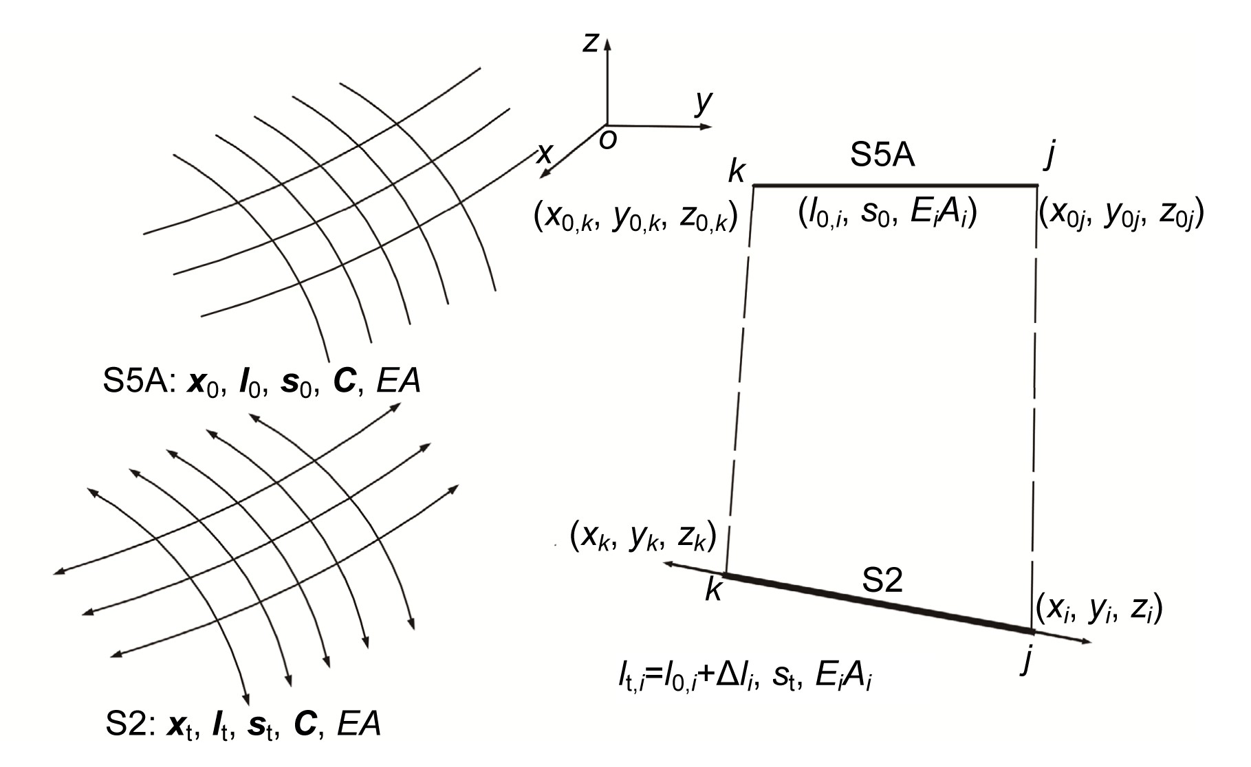
Let the vectors x, l, and s denote the configuration, cable length, and cable tension, respectively, where the subscript t represents the state S2 and subscript 0 represents the state S5A. For the cable-net structure, E is the elastic modulus, A is the cross-sectional area, and the matrix C is the connectivity matrix which defines the specific topology.
For a single cable link i and the cable-net structure, the mechanical description model is illustrated in Fig. 2 for the pre-stress release process P4A2 from state S2 to state S5A.
Fig.2 Pre-stress release procedure of a cable-net and one cable link i
The unstressed length l0,i of the link i can be formulated as
,
where, for link i, Ei is the elastic modulus, Ai is the cross-sectional area, lt,i is the stressed cable length and st,i is the cable tension.
Then the elongation of the link i can be written as
.
By calculating the unstressed length and elongation for all cable links, the unstressed length vector l0 and the elongation vector v(Δl) of the cable-net structure are obtained.
2.1.2. Optimal LNLS approach
In this study, the governing equations are developed for the pre-stress release analysis which is an inverse solution. Consider a free joint j connected with joints h and k in a cable-net assembly (Fig. 3), the equilibrium equation of joint j can be expressed as
where s is the cable tension, l is the force cable length, and p is the external load.
Fig.3 Joint equilibration state in a cable-net
Considering a cable-net structure with n joints and m cables, the global equilibrium equation can be written in the matrix form:
,
where is the equilibrium matrix, is the cable tension vector, and is the external load vector.
Similarly, the compatibility equation can be established as follows:
,
where () is the compatibility matrix, is the joint displacement vector, and is the elongation vector of the cables.
According to the matrices theory, when the number of equations m is less than the number of variables 3n, the solution to Eq. (5) can be expressed as follows (Nashed, 1976):
,
where Null(B) is the basis for the nullspace of the compatibility matrix B, is the Moore-Penrose inverse, is a vector consisting of the participation coefficients of the mechanisms, and r is the rank of B.
The second part of Eq. (6) results in infinite solutions, which is not only independent from the cable elongation but also orthogonal to the first part. To obtain the optimal solution, some constraints should be supplemented. In general, and the property of the matrix norm is . The LNLS is assumed, thus the solution to Eq. (5) is
,
which implies that the movement mechanism is excluded in Eq. (7). Therefore, the cable-net structure is a first-order infinitesimal mechanism (Calladine and Pellegrino, 1991; Vassart et al., 2000). It is valid for small deformations near the equilibrium state; moreover, the deformation is minimal with a given elongation and the work of the external force is minimal relative to the joint displacement in terms of physical meaning.
2.1.3. Numerical iterative method and implementation
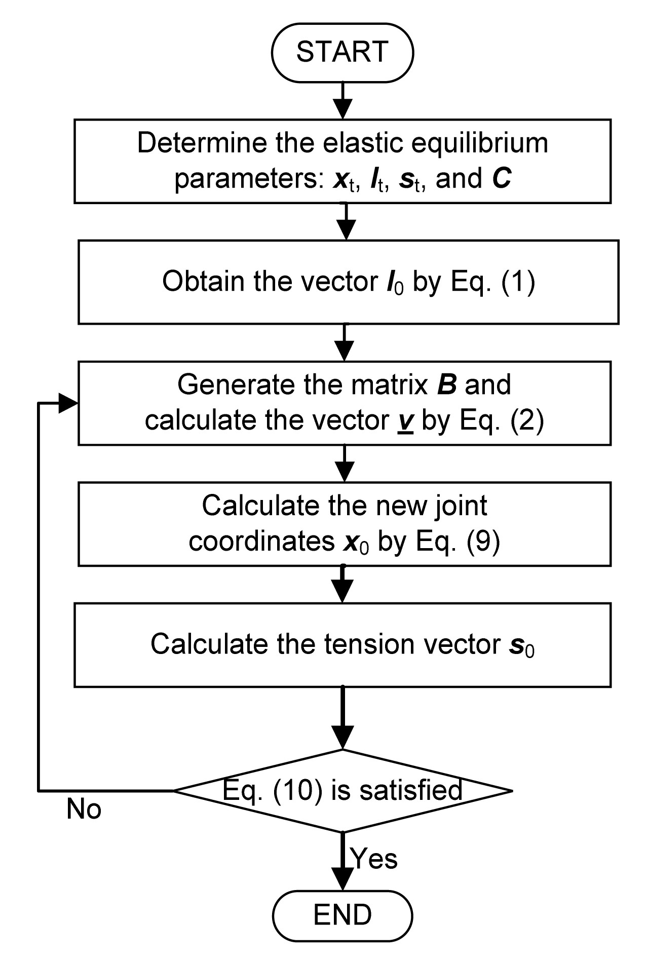
At first, the unstressed length vector l0 and the elongation vector can be calculated from Eqs. (1) and (2), respectively. Then the joint displacement can be computed from Eq. (7) after the compatibility matrix B is determined. Based on the above formulation, a numerical iterative method can be developed to perform pre-stress release procedures.
The configuration of the cable link assembly, i.e., the joint coordinates, can be updated by
.
Substituting Eq. (7) into Eq. (8), the configuration of the zero-stress state can be expressed as
.
It is an inverse operation from the elastic equilibrium state to the zero-stress state, in terms of physical meaning, the zero-stress state is the shortening of the cable link from the stressed state. Therefore, the components of vector in Eq. (9) should be negative corresponding to the shortening of the cable link from the zero-stress state to the stressed state.
Theoretically the elements of the tension vector s0 should all be zero in the zero-stress state, correspondingly the convergence criterion of the numerical calculation employed is
,
where |*| is the absolute value of the components of the vector, the function max(*) is the maximum value of the components of the vector, and ε is the convergence threshold value.
If Eq. (9) cannot be satisfied in the current state, the matrix B and vector should be regenerated in the current state, and the new configuration should be iteratively updated. When the convergence criterion is finally satisfied, the zero-stress state will be obtained.
Based on the proposed iterative procedure, a Matlab algorithm is developed and the flow chart of the computation of the pre-stress release analysis is shown in Fig. 4.
Fig.4 Flow chart of the computation of the pre-stress release analysis
In fact, the pre-stress release procedure is realized by releasing particular boundary constraints. As different release methods could result in different zero-stress states, even though some methods cannot completely release the pre-stress state, there is a need to investigate the pre-stress release method using the minimum constraints to release the pre-stress completely and effectively limit the global rigid movement. In addition, this case illustrates the non-unique solution of the inverse problem.
2.2. Computational methods for the S6A pre-stress state
Since cables can only carry tension in the process of load transfer, the cable-net structure has to be pre-tensioned on site to activate geometric stiffness so that cables can carry compression by reducing pre-tension. The resulting configuration and pre-stress is the “actual” pre-stress rather than the prescribed pre-stress.
Based on the S5A zero-stress state, the calculation of the pre-stress state S6A is a positive problem. Contrary to the pre-stress release analysis P4A2, this procedure is named pre-tensioning analysis P5A, as well as the intermediate procedures P5A1 and P5A2. Due to the existence of internal mechanisms (Calladine and Pellegrino, 1991), a standard nonlinear finite element (FE) approach to this problem inevitably involves a singular system matrix. Firstly, to overcome the initial singularity of the stiffness matrix, a feasible self-stress model is adopted in this study. Then an iterative nonlinear analysis procedure is developed based on the particular formulation of the cable link.
2.2.1. Governing equations
For the cable-net structure with m elements and nf free joints, the total potential energy function can be established, as follows (Ströbel, 1997):
,
where v, s, and x are independent unknowns; is the elastic strain energy of the cable links; is the external force potential energy; is the element elongation vector; is the element tension vector; is the element unstressed length vector; is the external conservative load vector excluding the boundary pretension force, which is independent from the configuration; is the vector of the joint coordinates in the current state, i.e., the current configuration; is the coordinate vector in the unstressed state, i.e., the initial configuration; f(x) is the cable link length function with respect to , which is identical to the element stressed length vector in the current state; and is a diagonal matrix of the element stiffness whose diagonal entry is kii=EiAi/l0i.
Calculating the derivative of the total potential energy with respect to x, , and s, respectively, and then setting them all equal to zero, the equilibrium, constitutive, and compatibility equations of the structure can be obtained as follows:
,
,
.
Using the Taylor expansion of the equilibrium equation and neglecting the second-order term, Eq. (12a) can be formulated into:
.
By introducing the Jacobian matrix ∂f(x)/∂x=Ā, Eq. (13) can be simplified into:
,
where the global stiffness matrix G consists of two parts: the elastic stiffness , and the geometric stiffness Z.
The cable link length function fi(x) of the cable link i with start joint k and end joint j is written as
.
The derivative of fi(x) with respect to x is
.
The elastic stiffness matrix of the element i can be written as
.
In addition,
.
Solving the second-order derivative of fi(x) and multiplying the elemental tension si, the geometric stiffness matrix of the element i can be obtained as shown in Eq. (19):
With the linearization of Eq. (12c), the vector of the element elongation can be written as
,
where is a known vector of the elemental elongation.
To assemble the global stiffness matrix G, the elastic stiffness and geometric stiffness for all cable links could be calculated by Eqs. (17) and (18), respectively. Normally the matrix G is non-singular due to the existence of geometric stiffness. Therefore, substituting Eq. (20) into Eq. (14), the basic equation of the pre-tensioning analysis by moving boundary joints can be obtained as
.
Although Eq. (21) provides an approach to the movement increment Δx of the boundary joints in the pre-tensioning process, it is invalid when the matrix is singular. In other words, Eq. (21) cannot be temporarily solved in the initial unstressed state, since the initial stiffness matrix G is non-invertible without introducing the geometric stiffness.
2.2.2. Initial tension of the feasible self-stress model
To avoid the singularity of the initial stiffness matrix G, a small assumed initial tension is used to activate a certain geometric stiffness in the cable link structure. Therefore, Eq. (21) can be simulated at an assumed state which is infinitely close to the initial unstressed state. A feasible self-stress mode, in which all elements are greater than zero corresponding to all cables being under tension, is adopted as the assumed initial tension to ensure that the system satisfies equilibrium in the current state.
As illustrated in the matrix analysis, the null-space of A contains the self-stress modes which are element forces in the absence of an external load. The solution to find the bases for the null-space is not unique. The Gaussian elimination method is efficient but it has problems with handling matrices which are rank-deficient, while singular value decomposition (SVD) is a little time-consuming but robust and stable due to the orthogonal transformation. Herein we capitalize on SVD, in which the matrix A can be expressed as
,
where is the non-zero singular value of matrix A, is the left orthogonal matrix, is the right orthogonal matrix, and r is the rank of matrix A.
The singular value matrix satisfies:
According to the above formula, the matrix W can be partitioned into two parts:
.
Thus, .
According to Eqs. (23) to (25), the following can be obtained:
.
As indicated in Eq. (26), the columns of matrix are the orthogonal bases for the nullspace of matrix A. In other words, the self-stress modes can be given by the matrix . If there is a self-stress mode where all the elements are greater than zero, it is a feasible self-stress mode which can be interpreted as the assumed initial tension . If there is no feasible self-stress mode, the initial tensile forces of all the elements should be assumed to be very small (e.g., 1 N). The assumed unstressed length vector at the zero-stress state can then be calculated using Eq. (1).
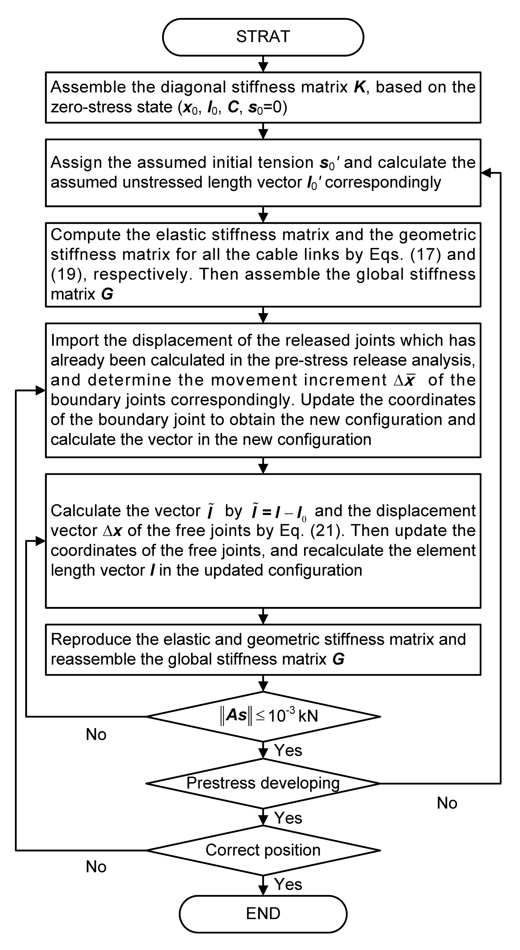
2.2.3. Computational procedure and implementation
In this pre-tensioning analysis P5A, the computational method imports a small assumed initial tension to avoid the singularity of the initial stiffness matrix G. Due to this import of assumed initial tension, the real theoretical unstressed state changes correspondingly. To eliminate this effect, the element length l0 at the initial unstressed state is always taken as the real unstressed length.
As shown in Fig. 5, the computational procedure is summarized and the corresponding Matlab algorithm is developed to implement the pre-tensioning analysis.
Fig.5 Flow chart of the computation of the pre-tensioning development analysis
In the iterative computation process, the release movement of boundary joints is discretized into small increments. In the calculation of the incremental movement, the pre-tensioning development can be determined step by step. In other words, the tension and the configuration can be evaluated step by step. The calculation stops when the released joints are moved to the expected position of the elastic equilibrium state. Finally, the pre-stressed state S6A is achieved.
In the actual construction process of cable-net structures, the boundary joints can be stretched in different sequences (e.g., synchronously or non-synchronously). Moreover, different movement imports of boundary joints can be adopted to simulate the actual pre-tensioning process. The intermediate configuration S7A can be obtained through the intermediate pre-tensioning processes P5A1 and P5A2. In addition, the pre-tensioning force of boundary links is dependent on configuration, which could be used to choose and control the hydraulic jack.
3. Numerical examples
To demonstrate the pre-stress release and pre-tension analysis, two typical examples are given based on the aforementioned algorithms. Moreover, two distinct methods have been performed to investigate the structural behavior in this analysis.
3.1. Diamond cable-net example
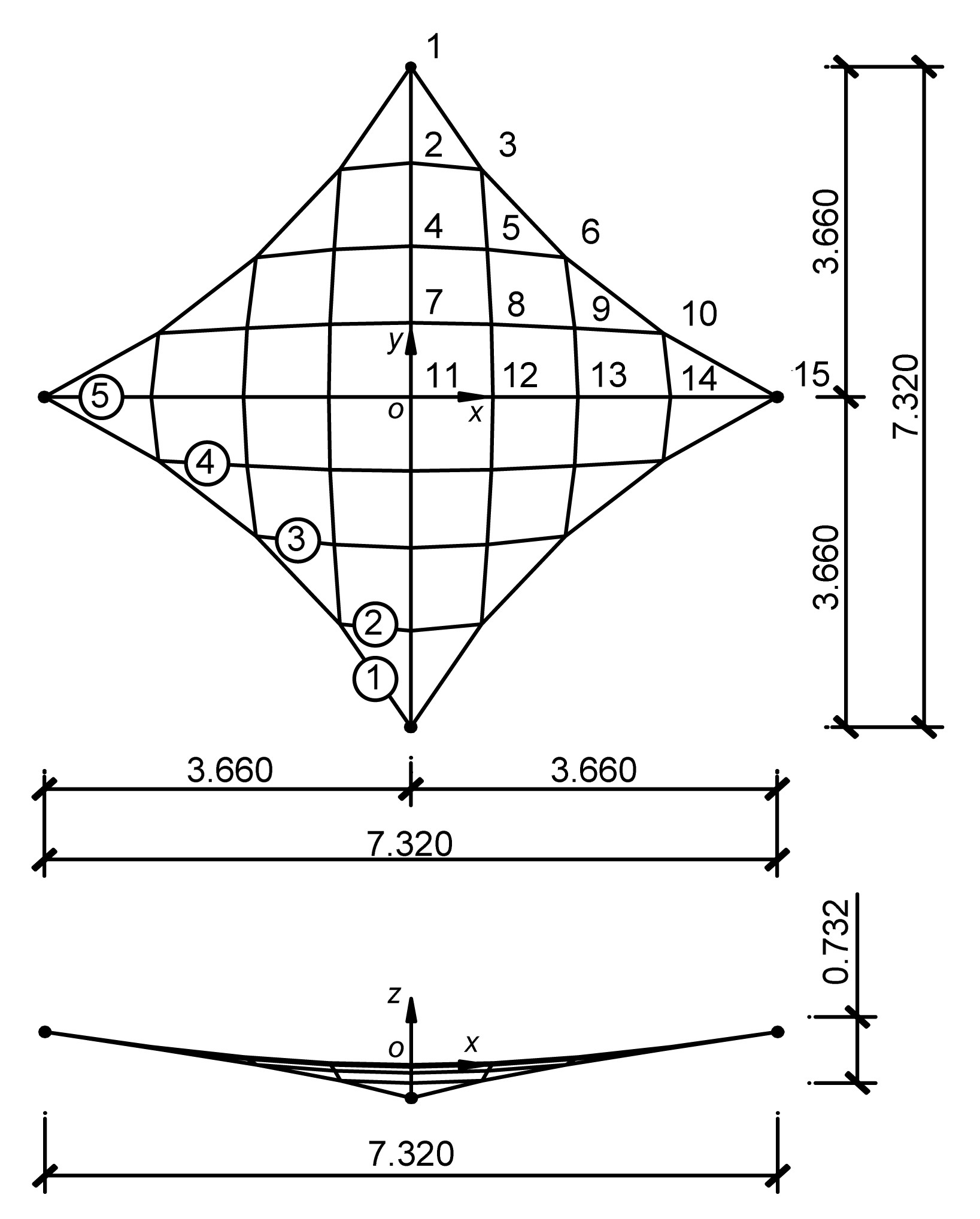
As shown in Fig. 6, the diamond cable-net consists of 41 joints and 80 cable links with four fixed corner joints. The lower corner joints are joint 1 and its symmetrical joint, while the upper one is joint 15 and its symmetrical joint. The plan is 7.32 m×7.32 m, and the difference in elevation between the upper joint and the lower joint is 0.732 m. Due to symmetry, only the data of joints 1 to 15 are detailed in this example.
Fig.6 Equilibrium configuration of form finding (unit: m)
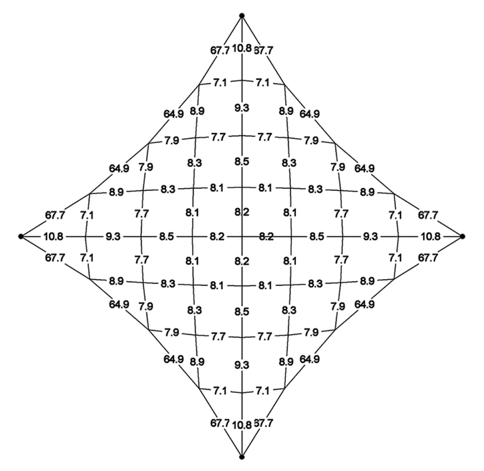
Based on the force density method, the form of this structure was formed with a 50 kN/m force density in the boundary cables and a 10 kN/m force density in the inner cables. The material was assigned to the members, where the cross-section stiffness of the boundary cables was EA=15 000 kN, and that of the inner cables was EA=3000 kN. In the absence of external loads and self-weight, the distribution of tension is shown in Fig. 7.
Fig.7 Distribution of tension at the equilibrium state S2 (unit: kN)
3.1.1. Computation of zero-stress state S5A
Based on the equilibrium state S2, the theoretical zero-stress state S5A can be achieved using two different pre-stress release methods: the four fixed joints release and the two lower fixed joints release.
1. Four fixed joints release
In the first method, the constraint in the y and z directions of the lower corner points and the constraints in the x and z directions of the upper one are released. When the convergence criterion is set at kN, the zero-stress state can be obtained after only three iterations, which demonstrates the effectiveness of the aforementioned algorithm.
The configuration and the displacements obtained by the developed algorithm are listed in Table 1, and those obtained by the dynamic relaxation method (DRM) (Zhao et al., 2012) are also listed in Table 2 for comparison. As anticipated, the results are in good agreement with those of DRM, which demonstrates the correctness of the algorithm. As illustrated in Table 1, the central joint 11 remained unchanged, and the others symmetrically retracted with respect to the x=0 and y=0 planes.
Table 1
Coordinates and displacements of joints 1 to 15 (four fixed joints release)
Joint No.
Equilibrium state S2
Zero-stress state S5A
Zero-stress state S5A (DRM)
Displacement (mm)
x (m)
y (m)
z (m)
x (m)
y (m)
z (m)
x (m)
y (m)
z (m)
∆x
∆y
∆z
1
0.000
3.660
−0.366
0.000
3.646
−0.356
0.000
3.646
−0.358
0
−14
10
2
0.000
2.594
−0.201
0.000
2.588
−0.167
0.000
2.588
−0.168
0
−6
35
3
0.708
2.521
−0.175
0.706
2.515
−0.158
0.706
2.515
−0.159
−1
−6
17
4
0.000
1.671
−0.089
0.000
1.668
−0.058
0.000
1.668
−0.058
0
−3
31
5
0.765
1.636
−0.066
0.763
1.633
−0.045
0.763
1.633
−0.044
−2
−3
21
6
1.545
1.545
0.000
1.543
1.543
0.000
1.543
1.543
0.000
−2
−2
0
7
0.000
0.820
−0.022
0.000
0.818
−0.010
0.000
0.819
−0.010
0
−2
12
8
0.805
0.805
0.000
0.803
0.803
0.000
0.803
0.803
0.000
−2
−2
0
9
1.636
0.765
0.066
1.633
0.763
0.045
1.633
0.763
0.044
−3
−2
−21
10
2.521
0.708
0.175
2.515
0.706
0.158
2.515
0.706
0.159
−6
−1
−17
11
0.000
0.000
0.000
0.000
0.000
0.000
0.000
0.000
0.000
0
0
0
12
0.820
0.000
0.022
0.818
0.000
0.010
0.819
0.000
0.010
−2
0
−12
13
1.671
0.000
0.089
1.668
0.000
0.058
1.668
0.000
0.058
−3
0
−31
14
2.594
0.000
0.201
2.588
0.000
0.167
2.588
0.000
0.168
−6
0
−35
15
3.660
0.000
0.366
3.646
0.000
0.356
3.646
0.000
0.358
−14
0
−10
2. Two lower fixed joints release
In the second method, the pre-stress release analysis is carried out by releasing the constraints in the y and z directions of the lower corner points. When the convergence criterion is set to , the theoretic zero-stress state can be obtained after only five iterations, which also demonstrates the effectiveness of the algorithm.
The configuration and the displacement obtained by the developed algorithms are listed in Table 2, and the results of DRM are also listed in Table 2 for comparison. As illustrated in Table 2, the central joint 11 is found at the left, and the other joints symmetrically retracted with respect to the x=0 and y=0 planes. It is found that the displacement in Table 2 was much greater than that in Table 1.
Table 2
Coordinates and displacements of joints 1 to 15 (two lower fixed joints release)
Joint No.
Equilibrium state S2
Zero-stress state S5A
Zero-stress state S5A (DRM)
Displacement (mm)
x (m)
y (m)
z (m)
x (m)
y (m)
z (m)
x (m)
y (m)
z (m)
∆x
∆y
∆z
1
0.000
3.660
−0.366
0.000
3.631
−0.344
0.000
3.630
−0.347
0
−29
22
2
0.000
2.594
−0.201
0.000
2.580
−0.117
0.000
2.579
−0.122
0
−14
84
3
0.708
2.521
−0.175
0.706
2.504
−0.124
0.706
2.503
−0.127
−2
−18
50
4
0.000
1.671
−0.089
0.000
1.666
0.035
0.000
1.666
0.033
0
−5
124
5
0.765
1.636
−0.066
0.763
1.631
0.046
0.763
1.630
0.039
−2
−5
112
6
1.545
1.545
0.000
1.544
1.537
0.062
1.544
1.536
0.056
−1
−8
62
7
0.000
0.820
−0.022
0.000
0.818
0.110
0.000
0.819
0.116
0
−2
132
8
0.805
0.805
0.000
0.803
0.803
0.125
0.803
0.803
0.128
−2
−2
125
9
1.636
0.765
0.066
1.633
0.763
0.168
1.633
0.763
0.170
−3
−2
102
10
2.521
0.708
0.175
2.521
0.706
0.219
2.522
0.706
0.216
0
−1
44
11
0.000
0.000
0.000
0.000
0.000
0.122
0.000
0.000
0.119
0
0
122
12
0.820
0.000
0.022
0.818
0.000
0.132
0.819
0.000
0.130
−2
0
110
13
1.671
0.000
0.089
1.669
0.000
0.166
0.169
0.000
0.169
−2
0
78
14
2.594
0.000
0.201
2.592
0.000
0.243
2.592
0.000
0.241
−2
0
42
15
3.660
0.000
0.366
3.660
0.000
0.366
3.660
0.000
0.366
0
0
0
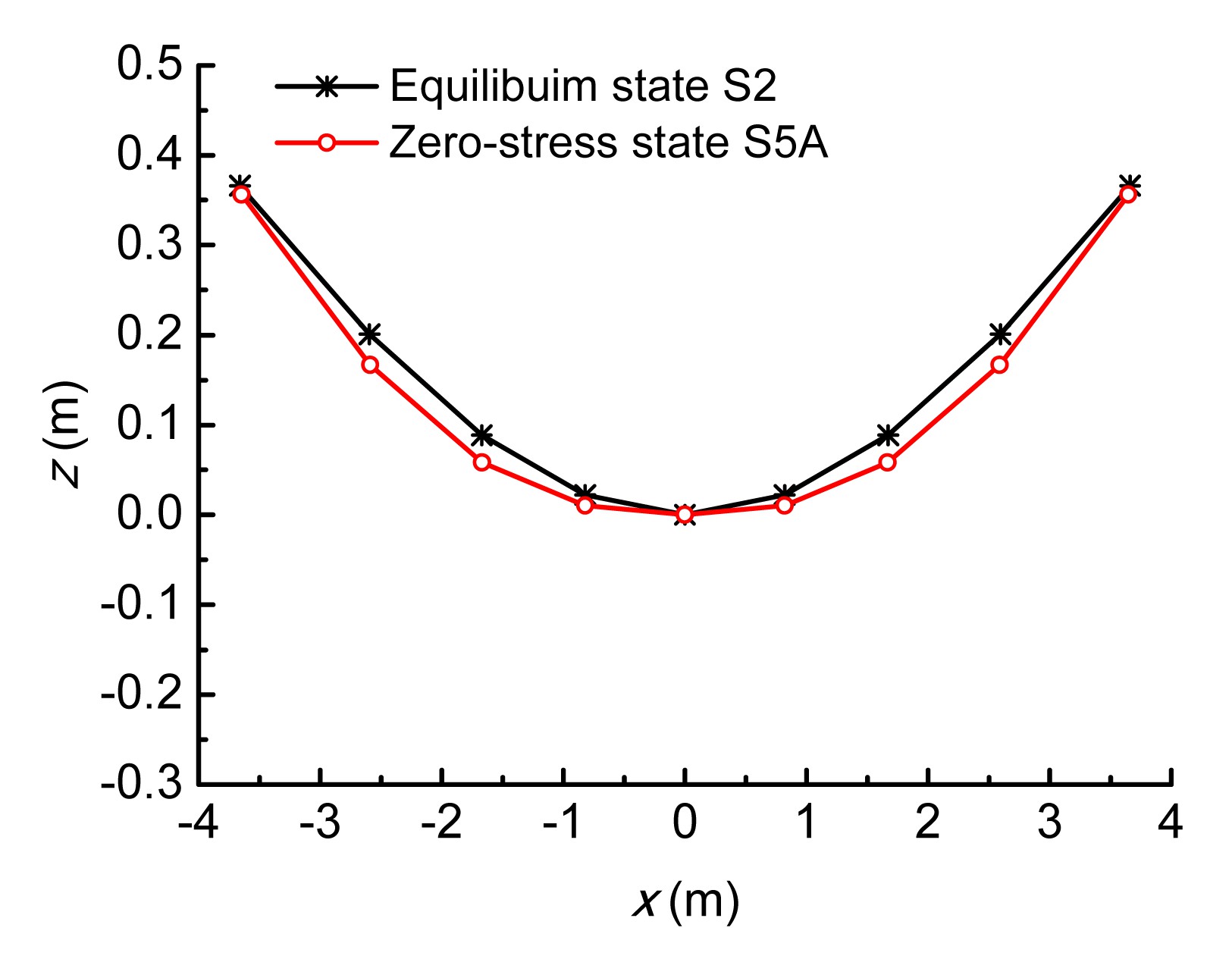
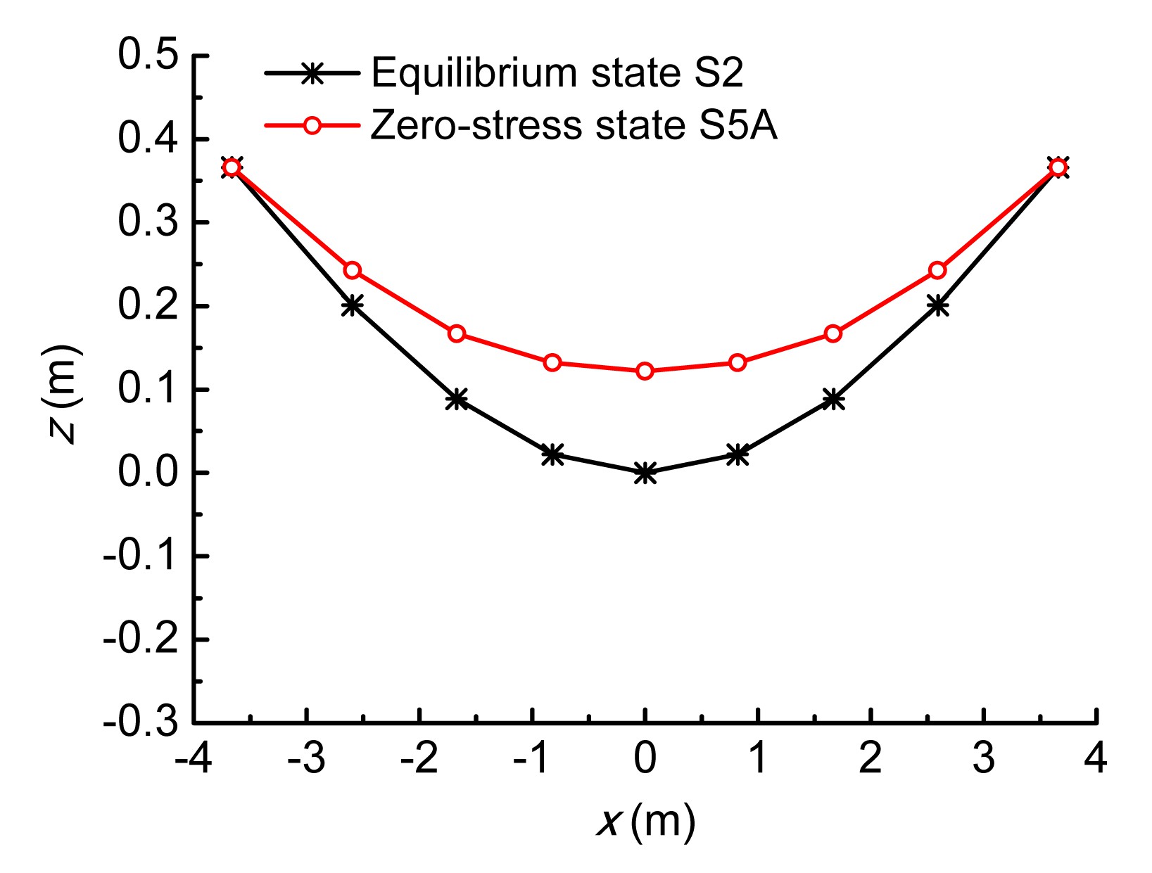
Fig. 8 (p.824) plots the cable shape at y=0 obtained by the first method, while Fig. 9 (p.824) shows the results obtained by the second method. Comparing Fig. 8 and Fig. 9, there are considerable differences between the cable shapes in the zero-stress states. Similar property is observed by comparing the configurations of joints in Table 1 and Table 2, which means that different methods of pre-stress release could result in different zero-stress states. In other words, the zero-stress state for the equilibrium state is not unique, which implies that the cable structures can be constructed in various ways.
Fig.8 Cable shape at y=0 (four fixed joints release)
Fig.9 Cable shape at y=0 (two lower fixed joints release)
3.1.2. Pre-tensioning development analysis
Based on the zero-stress state S5A, the pre-tensioning development analysis herein is conducted in two different methods: the first method is moving four released joints synchronously; the second one is moving two released lower joints synchronously. The movement direction of each joint is opposite to that of the corresponding displacement which is achieved in the above pre-stress release analysis. The displacement is divided into five equal increments, which means the pre-tensioning development is completed in five steps.
1. Moving four released joints synchronously
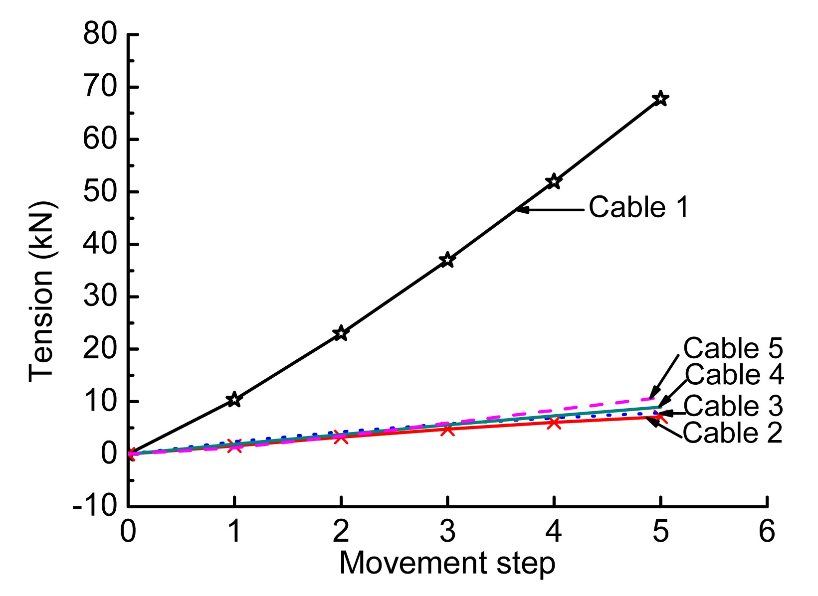
Taking the equilibrium convergence criterion, the joint unbalance force kN, and the changes of tension in cables 1 to 5 during the pre-tensioning development process are illustrated in Fig. 10. The configuration coordinates of joints in equilibrium state S2 and the “actual” pre-stressed state S6A are listed in Table 3 with three decimals. As indicated in Table 3, there is no obvious difference between these two states, which means that state 6A is the same as state S2.
Fig.10 Change of tension in cables 1–5 (moving four released joints synchronously)
Table 3
Coordinates and differences of joints 1 to 15 (unit: m)
Joint No.
Equilibrium state S2
Actual pre-stressed state S6A
x
y
z
x
y
z
1
0.000
3.660
−0.366
0.000
3.660
−0.366
2
0.000
2.594
−0.201
0.000
2.594
−0.201
3
0.708
2.521
−0.175
0.708
2.521
−0.175
4
0.000
1.671
−0.089
0.000
1.671
−0.089
5
0.765
1.636
−0.066
0.765
1.636
−0.066
6
1.545
1.545
0.000
1.545
1.545
0.000
7
0.000
0.820
−0.022
0.000
0.820
−0.022
8
0.805
0.805
0.000
0.805
0.805
0.000
9
1.636
0.765
0.066
1.636
0.765
0.066
10
2.521
0.708
0.175
2.521
0.708
0.175
11
0.000
0.000
0.000
0.000
0.000
0.000
12
0.820
0.000
0.022
0.820
0.000
0.022
13
1.671
0.000
0.089
1.671
0.000
0.089
14
2.594
0.000
0.201
2.594
0.000
0.201
15
3.660
0.000
0.366
3.660
0.000
0.366
2. Moving two released lower joints synchronously
Taking the same equilibrium convergence criterion kN, the changes of tension in cables 1 to 5 during the pre-tensioning development process are illustrated in Fig. 11.
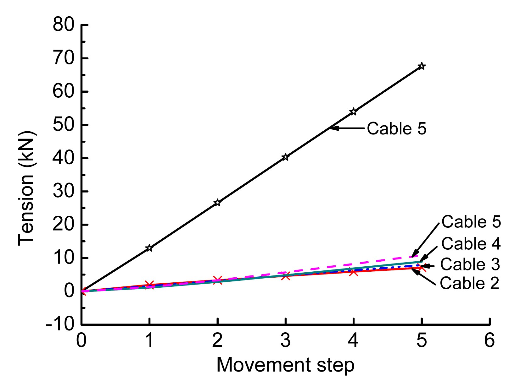
Fig.11 Variation of tension with movement increments in cables 1–5 (moving two released joints simultaneously)
As shown in Fig. 10, the trend of tension was approximately linear in the first movement step; however, it apparently became nonlinear in the second movement step. In these two movement steps, the relative tension deviations between the “actual” pre-stressed state S6A and the equilibrium state S2 were all less than 0.2%. According to the data expressed with three decimals in Table 3, the configurations of the joints in the state S6A are identical to those in the state S2. Therefore, the “actual” pre-stressed state can be realized using the intermediate state, namely, the theoretical zero-stress state. In other words, combining the pre-stress release and pre-tensioning development analyses together could successfully eliminate the shape and pre-stress discrepancy.
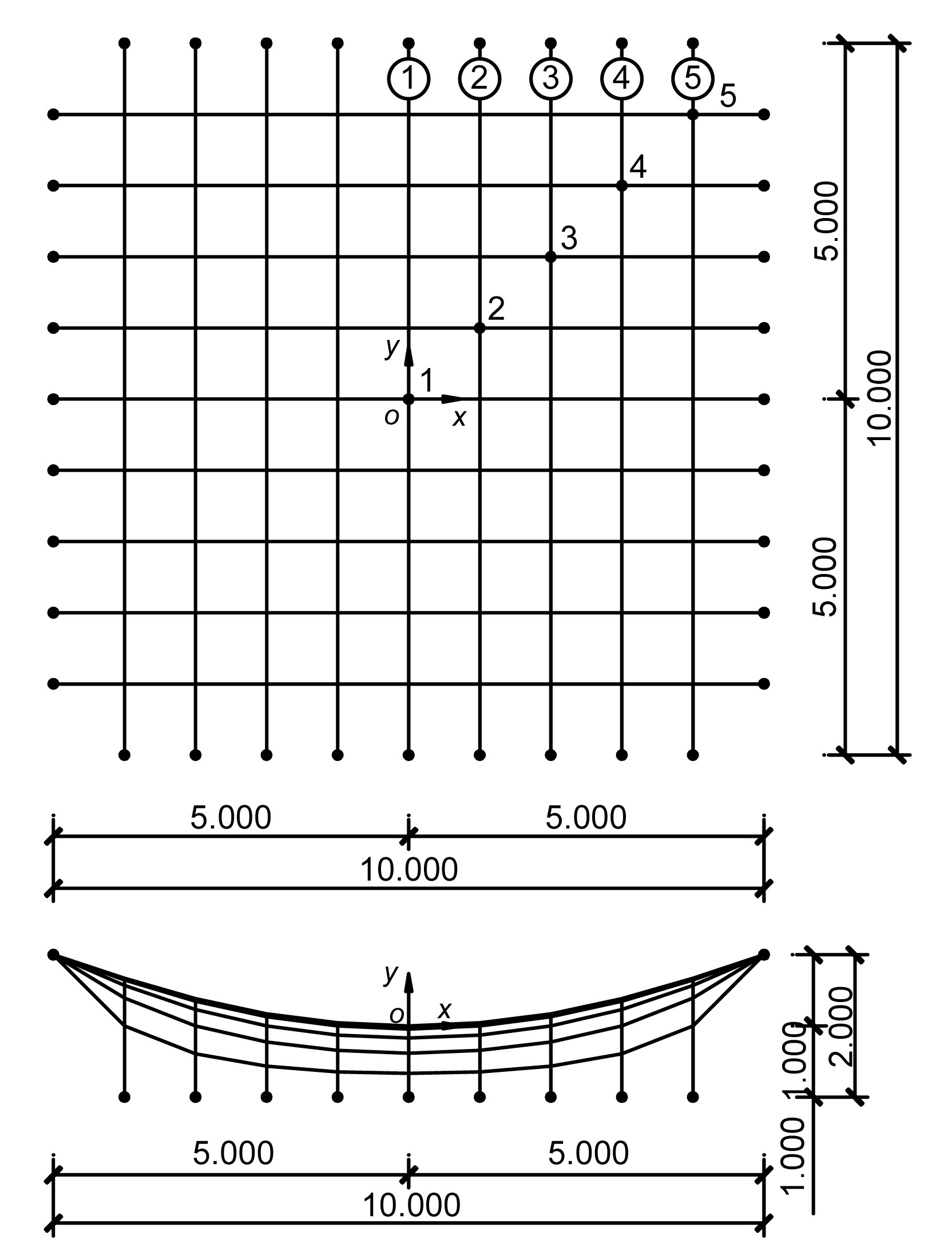
3.2. Rectangular cable-net example
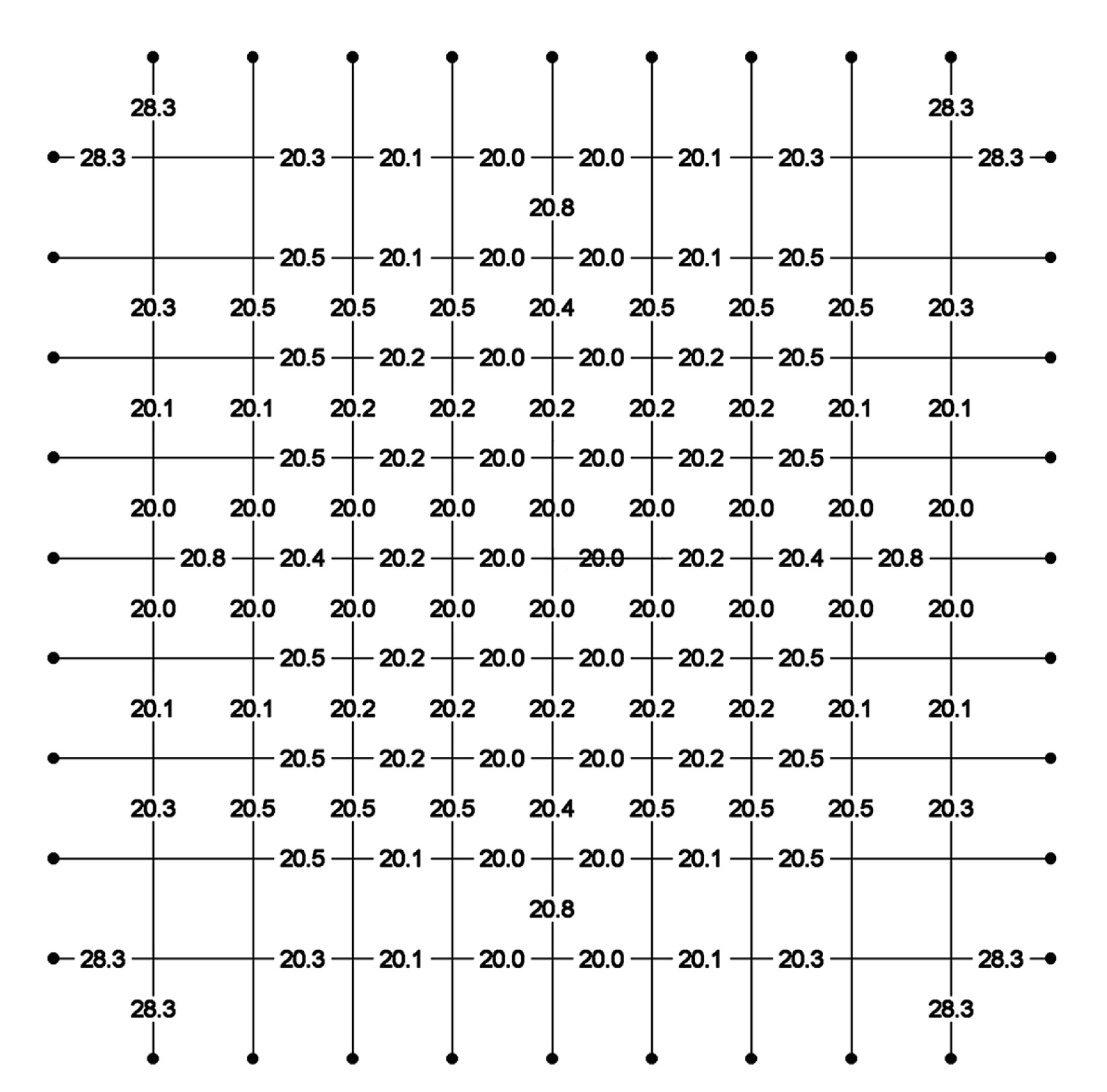
As shown in Fig. 12, the rectangular cable-net consists of 117 joints and 180 cable links. The grid size is 1 m×1 m, the plan is 10 m×10 m, and the elevation difference is 2 m. Based on the force density method, the form of this structure was formed with a 20 kN/m force density in all the cables. The section stiffness EA=5000 kN was assigned to all the cables. In the absence of external loads, the tension distribution of the main cables is shown in Fig. 13.
Fig.12 Equilibrium configuration of form finding (unit: m)
Fig.13 Tension distribution of main cables at the equilibrium state (unit: kN)
The theoretical zero-stress S5A is evaluated by releasing the constraints in the y and z directions of all lower boundary fixed joints at both sides. Based on this zero-stress state, the corresponding pre-tensioning development analysis is conducted by moving all the released lower fixed joints. The direction of movement of each joint is opposite to that of the corresponding joint displacement. Every displacement is divided into five equal movement increments. Because the displacements of the joints were different, the movement increments of the joints were not identical to each other.
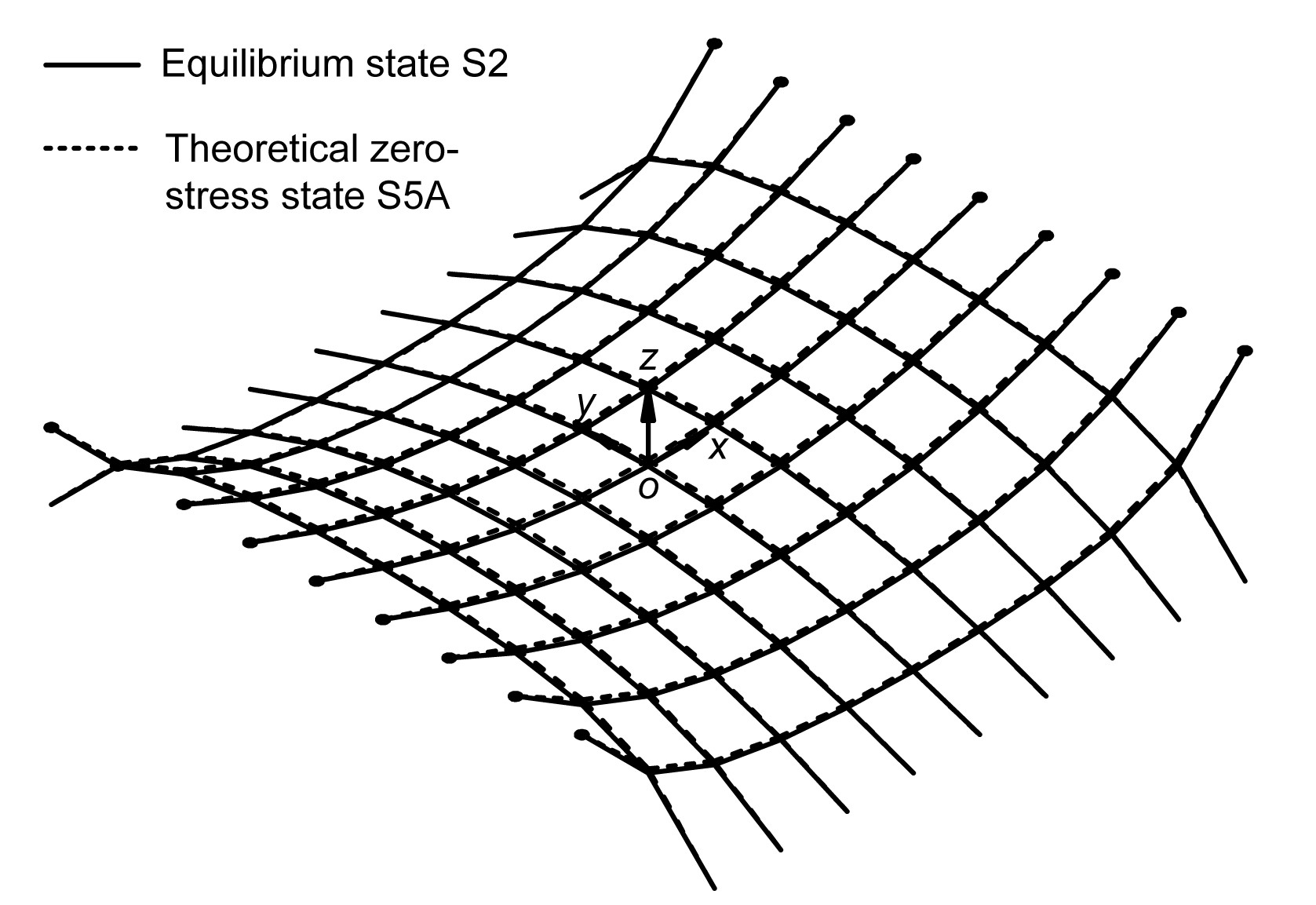
Taking the residual tension of cable link as the convergence criterion, the theoretical zero-stress state S5A can be obtained after three iterations. The change of configuration from equilibrium state S2 to the theoretical zero-stress state S5A is shown in Fig. 14, in which the solid line is equilibrium state S2, and the dashed line is the theoretical zero-stress state S5A.
Fig.14 Perspective view at equilibrium state S2 and zero-stress state S5A
Taking the joint unbalance force kN as the equilibrium convergence criterion, the changes of tension in cables 1 to 5 during the pre-tensioning development process are illustrated in Fig. 15. The coordinates of joints 1 to 5 in the equilibrium state S2, zero-stress state S5A, and the “actual” pre-stressed state S6A are listed in Table 4 with three decimals. It is apparent that the coordinates of the state S2 and the state S6A are virtually identical.
Fig.15 Change of tension in cables 1 to 5 during the pre-tensioning development process
Table 4
Coordinates of joints 1 to 5 (unit: m)
Joint No.
Equilibrium state S2
Zero-stress state S5A
Pre-stressed state S6A
x
y
z
x
y
z
x
y
z
1
0.000
0.000
0.000
0.000
0.000
0.078
0.000
0.000
0.000
2
1.000
1.000
0.000
0.996
0.996
0.071
1.000
1.000
0.000
3
2.000
2.000
0.000
1.991
1.990
0.057
2.000
2.000
0.000
4
3.000
3.000
0.000
2.985
2.984
0.045
3.000
3.000
0.000
5
4.000
4.000
0.000
3.978
3.978
0.035
4.000
4.000
0.000
As shown in Fig. 15, the change of tension became greater as the cable became closer to the boundary. In addition, the maximum relative deviation of the tension between the “actual” pre-stressed state S6A and the design equilibrium state S2 was barely 0.13%. According to the data expressed with three decimals in Table 4, the coordinates of the joints in the “actual” pre-stressed state S6A are identical to those at the equilibrium state S2.
4. Conclusions
According to the previous research, the common design concept for cable-net structures consists of two basic stages: the first is form finding and the second is static and dynamic analyses. Based on the equilibrium state of form finding, the static and dynamic analyses are carried out to investigate the structural behavior without introducing the influence of the pre-tensioning process. It has been discovered that this separation of design process is associated with the discrepancy in stress distribution and configuration between the numerically found structure and the real one.
Aimed at minimizing this highly non-uniform discrepancy, in this paper an extended design concept is proposed and the corresponding flow chart is simulated, suggesting a highly detailed description of the stress state and simulation procedure. Unlike the common design concept, this extended concept provides clear clarifications of mechanical behavior by considering the integrity of the design process, which means the form finding analysis, pre-stress release analysis, and pre-tensioning development analysis should be consecutively carried out.
In this paper, for the inverse problem from the equilibrium state of form finding S2 to the theoretical zero-stress state S5A in the pre-stress release analysis, an iterative computational method is developed, which capitalizes on the LNLS approach to the compatibility equation on account of the indeterminate nature of the cable-net structures. Moreover, for the positive problem from the S5A to the “actual” pre-stress state S6A in the pre-tensioning development analysis, another iterative computational method is developed by moving the boundary joints, in which the governing equations are explicitly formulated according to the particular energy function, and the feasible self-stress mode is adopted to avoid the singularity of initial stiffness matrix.
This study found that the configuration of the zero-stress state obtained herein compares well with those obtained by the dynamic relaxation method, which validates the efficiency and accuracy of our computational method. It also found that the “actual” pre-stress and configuration predicted by our computational methods are consistent with the prescribed pre-stress state, suggesting that the combination of the pre-stress release and pre-tensioning development analyses could successfully eliminate the shape and pre-stress discrepancies. In other words, this study has made some substantial progress in the elimination of the discrepancy; it also provides a superior and integral approach to the final pre-stress state and configuration. With this integral approach, a thorough numerical investigation for cable-net structures becomes available, even including the analysis of common wind-induced effects.
In addition, another improvement noted herein is that these computational methods are formulated as modular procedures in order to be a standard design process. As the realization of each design procedure is strongly affected by the underlying design problem, appropriate computer methods should be adopted. Most notably, all the aforementioned methods and their respective combinations are advanced tools that enable the realization of even more complicated and more challenging structures, which are definitely within the scope of modern tensile structure design.
[1] Argyris, J.H., Scharpf, D.W., 1972. Large deflection analysis of prestressed networks. Journal of the Structural Division, 98(3):633-654.
[2] Argyris, J.H., Angelopoulos, T., Bichat, B., 1974. A general method for the shape finding of lightweight tension structures. Computer Methods in Applied Mechanics and Engineering, 3(1):135-149.
[3] Ashwear, N., Eriksson, A., 2014. Natural frequencies describe the pre-stress in tensegrity structures. Computers & Structures, 138:162-171.
[4] Barnes, M., 1994. Form and stress engineering of tension structures. Structural Engineering Review, 6(3):
[5] Blanco-Fernandez, E., Castro-Fresno, D., Del Coz Diaz, J.J., 2011. Flexible systems anchored to the ground for slope stabilisation: critical review of existing design methods. Engineering Geology, 122(3-4):129-145.
[6] Blanco-Fernandez, E., Castro-Fresno, D., Del Coz Daz, J., 2013. Field measurements of anchored flexible systems for slope stabilisation: evidence of passive behaviour. Engineering Geology, 153:95-104.
[7] Bletzinger, K.U., Ramm, E., 1999. A general finite element approach to the form finding of tensile structures by the updated reference strategy. International Journal of Space Structures, 14(2):131-145.
[8] Bletzinger, K.U., Linhard, J., Wchner, R., 2010. Advanced numerical methods for the form finding and patterning of membrane structures. New Trends in Thin Structures: Formulation, Optimization and Coupled Problems, Springer,:133-154.
[9] Calladine, C., Pellegrino, S., 1991. First-order infinitesimal mechanisms. International Journal of Solids and Structures, 27(4):505-515.
[10] Castro-Fresno, D., Del Coz Diaz, J., Lpez, L., 2008. Evaluation of the resistant capacity of cable nets using the finite element method and experimental validation. Engineering Geology, 100(1-2):1-10.
[11] Chen, W.J., Zhang, L.M., 2008. Approximated zero-stress state based on structural analysis procedures for the cable structures. , International Symposium on Advances in Mechanics, Materials and Structures, Zhejiang University, Hangzhou, China, :
[12] Chen, W.J., Zhang, L.M., 2011. Elastified procedure for the form-found equilibrium state and zero-stress state of cable-net structure. Journal of Shanghai Jiao Tong University, (in Chinese),(45):523-527.
[13] Day, A., Bunce, J., 1970. Analysis of cable networks by dynamic relaxation. Civil Engineering Public Works Review, 4:383-386.
[14] Del Coz Diaz, J.J., Nieto, P.G., Fresno, D.C., 2009. Non-linear analysis of cable networks by FEM and experimental validation. International Journal of Computer Mathematics, 86(2):301-313.
[15] Eriksson, A., Tibert, A.G., 2006. Redundant and force-differentiated systems in engineering and nature. Computer Methods in Applied Mechanics and Engineering, 195(41-43):5437-5453.
[16] Grndig, L., Moncrieff, E., Singer, P., 2000. A history of the principal developments and applications of the force density method in Germany 1970–1999. , Fourth IASS-IACM International Colloquium on Computation of Shell & Spatial Structures, Chania-Crete, Greece, 1-13. :1-13.
[17] Haber, R., Abel, J., 1982. Initial equilibrium solution methods for cable reinforced membranes part II—implementation. Computer Methods in Applied Mechanics and Engineering, 30(3):285-306.
[18] Lewis, W., Jones, M., Rushton, K., 1984. Dynamic relaxation analysis of the non-linear static response of pretensioned cable roofs. Computers & Structures, 18(6):989-997.
[19] Linkwitz, K., Grutndig, L., 1987. Strategies of form finding and design and construction of cutting patterns for large sensitive membrane structures. , International Conference on the Design and Construction of Non-conventional Structures, 315-321. :315-321.
[20] Nashed, M.Z., 1976. Generalized Inverses and Applications: Proceedings of an Advanced Seminar, Academic Press,1973:
[21] Schek, H.J., 1974. The force density method for form finding and computation of general networks. Computer Methods in Applied Mechanics and Engineering, 3(1):115-134.
[22] Strbel, D., 1997. Die Anwendung der Ausgleichungs rechnung auf elastomechanische Systeme, (in Germany), Beck :
[23] Vassart, N., Laporte, R., Motro, R., 2000. Determination of mechanism’s order for kinematically and statically indetermined systems. International Journal of Solids and Structures, 37(28):3807-3839.
[24] Wagner, R., 2005. On the design process of tensile structures. Textile Composites and Inflatable Structures, Springer,:1-16.
[25] Zhao, J.Z., Chen, W.J., Fu, G.Y., 2012. Computation method of zero-stress state of pneumatic stressed membrane structure. Science China Technological Sciences, (in Chinese),55(3):717-724.
Open peer comments: Debate/Discuss/Question/Opinion


Open peer comments: Debate/Discuss/Question/Opinion
<1>