Affiliation(s):
1.
Key Laboratory of Geomechanics and Embankment Engineering of Ministry of Education, Hohai University, Nanjing 210098, China; moreAffiliation(s): 1.
Key Laboratory of Geomechanics and Embankment Engineering of Ministry of Education, Hohai University, Nanjing 210098, China; 2.
Geotechnical Centrifuge Facility, the Hong Kong University of Science and Technology, Hong Kong, China; less
Charles W. W. Ng. The state-of-the-art centrifuge modelling of geotechnical problems at HKUST[J]. Journal of Zhejiang University Science A, 2014, 15(1): 1-21.
@article{title="The state-of-the-art centrifuge modelling of geotechnical problems at HKUST", author="Charles W. W. Ng", journal="Journal of Zhejiang University Science A", volume="15", number="1", pages="1-21", year="2014", publisher="Zhejiang University Press & Springer", doi="10.1631/jzus.A1300217" }
%0 Journal Article %T The state-of-the-art centrifuge modelling of geotechnical problems at HKUST %A Charles W. W. Ng %J Journal of Zhejiang University SCIENCE A %V 15 %N 1 %P 1-21 %@ 1673-565X %D 2014 %I Zhejiang University Press & Springer %DOI 10.1631/jzus.A1300217
TY - JOUR T1 - The state-of-the-art centrifuge modelling of geotechnical problems at HKUST A1 - Charles W. W. Ng J0 - Journal of Zhejiang University Science A VL - 15 IS - 1 SP - 1 EP - 21 %@ 1673-565X Y1 - 2014 PB - Zhejiang University Press & Springer ER - DOI - 10.1631/jzus.A1300217
Abstract: Geotechnical centrifuge modelling is an advanced physical modelling technique for simulating and studying geotechnical problems. It provides physical data for investigating mechanisms of deformation and failure and for validating analytical and numerical methods. Due to its reliability, time and cost effectiveness, centrifuge modelling has often been the preferred experimental method for addressing complex geotechnical problems. In this ZENG Guo-xi Lecture, the kinematics, fundamental principles and principal applications of geotechnical centrifuge modelling are introduced. The use of the state-of-the-art geotechnical centrifuge at the Hong Kong University of Science and Technology (HKUST), China to investigate four types of complex geotechnical problems is reported. The four geotechnical problems include correction of building tilt, effect of tunnel collapse on an existing tunnel, excavation effect on pile capacity and liquefied flow and non-liquefied slide of loose fill slopes. By reporting major findings and new insights from these four types of centrifuge tests, it is hoped to illustrate the role of state-of-the-art geotechnical centrifuge modelling in advancing the scientific knowledge of geotechnical problems.
Darkslateblue:Affiliate; Royal Blue:Author; Turquoise:Article
Article Content
1. Introduction
In tackling some complex geotechnical problems, centrifuge modelling is often considered as a preferred experimental method. According to a survey conducted by the British Geotechnical Society in 1999, centrifuge modelling was ranked fifth in the list of the most important developments in geotechnics over the previous 50 years (Fig. 1). The ranking was based on responses from 68 geotechnical experts in academia, consulting, contracting and research organisations. It is clear from the survey that centrifuge modelling plays a key role in geotechnical engineering.
Fig.1 The great and the good of 50 years of geotechnics (from Ground Engineering, July 1999)
In this paper, the kinematics, fundamental principles, and principal applications of geotechnical centrifuge modelling are introduced. Modelling of four complex geotechnical problems by the state-of-the-art geotechnical centrifuge at the Hong Kong University of Science and Technology (HKUST), China is described. The four geotechnical problems are: correction of building tilt, effect of tunnel collapse on an existing tunnel, excavation effect on pile capacity, and liquefied flow and non-liquefied slide of loose fill slopes. New insights from these four types of tests are revealed and the role of state-of-the-art geotechnical centrifuge modelling in improving understanding of the complex geotechnical problems is illustrated.
2. Brief introduction to the development of centrifuge modelling
According to Craig (1995), the earliest idea of using a centrifuge to increase self-weight of a small scale model was developed by Phillips in Paris in 1896. He suggested using a centrifuge to solve bridge engineering problems, but no actual test was carried out at that time. After this innovative idea, centrifuge modelling was not pursued until Bucky (1931), who conducted centrifuge model tests at Columbia University in the USA to study the integrity of mine roof structures in rock. Almost at the same time, Pokrovsky and Davidenkov from the Union of Soviet Socialist Republics (USSR) used a centrifuge to investigate problems associated with embankment and slope instability in 1933. In the subsequent two decades (1940s–1960s), a number of geotechnical centrifuges were built in the USSR and applied to tackling various problems in soils and rocks (Joseph et al., 1988). During the same period, a few research projects were undertaken in the USA by Panek (1949) and Clark (late 1950s and early 1960s). Apart from the USA and the USSR, early research work was conducted using a centrifuge by Ramberg (1968) in Sweden to study gravity tectonics, as well as by Hoek (1965) in South Africa for mining engineering. Also in the mid-1960s, the first geotechnical centrifuge was built in China by the Yangtze Water Conservancy Institute (Cheney, 1988). In 1966, the first geotechnical centrifuge in the UK was developed at Cambridge University by Prof. Schofield, who subsequently continued his work at the University of Manchester Institute of Science and Technology, where he built a large centrifuge in 1969. In the early 1970s, Profs. Rowe and Roscoe constructed centrifuges at the University of Manchester and Cambridge University, respectively. Thereafter, many researchers from various countries such as Japan, Denmark, Netherlands, and France visited Cambridge University to study centrifuge modelling techniques and to setup centrifuge facilities in their own countries (Joseph et al., 1988). In the mid-1970s, there was a renewed interest in geotechnical centrifuge modelling in the USA (Joseph et al., 1988). Centrifuge modelling was adopted to simulate geophysical events and processes by Ramberg (1968) in Chicago, craters formed by near-surface nuclear explosions and planetary impact of large bodies by Schmidt (1976), and cyclic and dynamic testing of piles by Scott (1979).
After the 1980s, centrifuge modelling was recognised and well-received in many countries, especially Japan (Kimura, 1998). Since then, there has been a continuing increase in the number, size, and simulation capability of centrifuges over the world, particularly in the last ten years in China.
3. Kinematics of centrifuge modelling
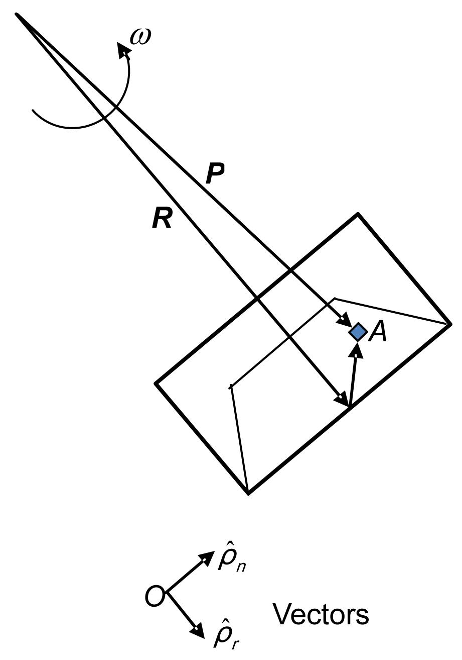
Fig. 2 shows plan view of a soil model in a spinning centrifuge. In this figure, a local Cartesian coordinate system (fixed to the model container) is defined.
Fig.2 Plan view of a soil model in a spinning centrifuge
Consider a soil element located at an arbitrary point A. At a given time, location of the arbitrary soil element A in the model container can be expressed as a vector summation:
,
where P and R denote vectors from axis of the centrifuge to soil element A and to the bottom of the model box (point O), respectively. R means a vector from point O to soil element A.
Acceleration of point A is
.
By assuming the centrifuge spins at a constant angular velocity (ω=constant, ) with a fixed radius of the centrifuge arm (|R|=constant), the acceleration of point A can be expressed as
.
According to their physical meanings, terms in Eq. (3) can be grouped into three parts as follows:
(1) denotes centripetal acceleration (due to spinning of centrifuge);
(2) describes the acceleration of a particle P relative to the centrifuge platform (e.g., resulting from applied base shaking, slope failure, explosions, etc.);
(3) refers to Coriollis acceleration (e.g., resulting from consolidation, flow, etc.).
Detailed derivations of the above equations are given by Lei and Shi (2003).
4. Fundamental principles of centrifuge modeling
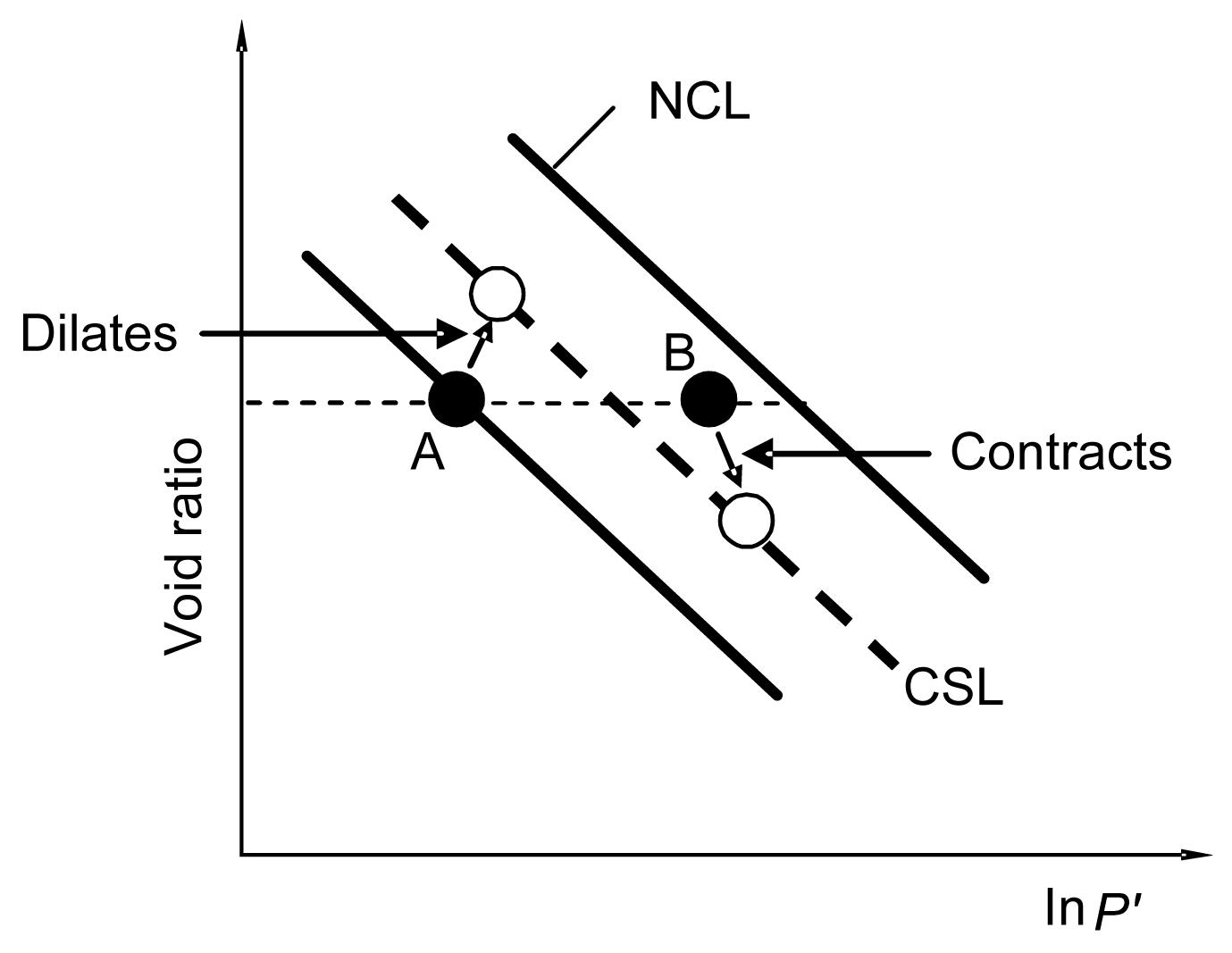
It is well recognised that soil behaviours are stress dependent. For an example illustrated in Fig. 3, a soil sample A located below the critical state line (CSL) initially, will dilate toward the CSL when it is sheared under a relatively low confining stress (e.g., in a small model test under one Earth’s gravity (i.e., 1g=9.81 m/s2)). By comparison, a sample, B, having the same density (i.e., same void ratio), located at an arbitrary point above the CSL but below or on the normal compression line (NCL), will contract when it is sheared under a higher mean effective stress, p' (i.e., high stress in the field or in the centrifuge). It is obvious that the use of test results from sample A for designing prototype problems is likely to be non-conservative and maybe even dangerous because the observed dilative behaviour at low stress under 1g conditions will not occur under high stress in the field. Thus, it is vital to simulate the stress level of the soil correctly before carrying out any physical experiment.
Fig.3 Distinct responses of two soil samples at the same density sheared under different confining stresses
The fundamental principle of centrifuge modelling is to recreate stress conditions, which would exist in a prototype, by increasing n times the “gravitational” acceleration in a 1/n scaled model in the centrifuge. Stress replication in the 1/n scaled model is approximately achieved by subjecting model components to an elevated “gravitational” acceleration, which is provided by centripetal acceleration (rω2=ng), where r and ω are the radius and angular velocity of the centrifuge, respectively. Thus, a centrifuge is suitable for modelling stress-dependent geotechnical problems. Apart from the ability to replicate in-situ stress level in a reduced size model in a centrifuge, one of the side benefits of centrifuge modelling is that the use of a small scale model shortens drainage paths of soil, resulting in a significant reduction of consolidation time by 1/n2.
For centrifuge model tests, scaling laws are generally derived through dimensional analysis, from the governing equations for a phenomenon, or from the principles of mechanical similarity between a model and a prototype (Taylor, 1995; Garnier et al., 2007). Some common scaling factors derived and used are summarised in Table 1.
Table 1
Some common scaling factors for centrifuge tests
Parameter
Scale factor (model/prototype)
Acceleration
n
Linear dimension
1/n
Stress
1
Strain
1
Mass
1/n3
Density
1
Unit weight
n
Force
1/n2
Bending moment
1/n3
Bending moment/unit width
1/n2
Flexural stiffness
1/n4
Flexural stiffness/unit width
1/n3
Time (dynamic)
1/n
Time (consolidation/diffusion)
1/n2
Time (creep)
1
Pore fluid velocity
n
Velocity (dynamic)
1
Frequency
n
5. Principal applications of centrifuge modelling
According to Ko (1988), four principal applications of geotechnical centrifuges can be classified as follows.
5.1. Modelling of prototype
Modelling of prototype is an obvious and direct application of the centrifuge modelling technique to simulate and tackle actual engineering problems. Some common applications include investigating slope instability, pile capacity, and the effect of tunnelling/excavation on adjacent existing underground structures. Both qualitative and quantitative analyses are possible from model tests.
5.2. Investigation of new phenomena
Centrifuge modelling has been successfully applied to the study of various unusual phenomena that are not well understood and are extremely difficult to study. Typical examples include plate tectonics, crater formations by nuclear explosions, various earthquake-induced events and soil liquefaction, and transportation of contaminants in soil. Behaviour of loose-fill slopes subjected to various rainfall and earthquake conditions can also be investigated.
5.3. Parametric studies
Parametric study in geotechnical centrifuge modelling is an example where physical model experiments are best rewarded. Normally, a major effort is necessary to design and manufacture the first model, while the actual testing and small variations in the model are relatively easily performed. By varying some model parameters (geometry, loading and boundary conditions, rainfall intensity or soil type), the sensitivity of test results to these variations can be evaluated and the most critical parameters can be identified. This leads directly to the possibility of generating useful design charts. Examples include bearing capacity of footings on slopes, critical design parameters in flow processes, and capacity of laterally loaded pile groups.
5.4. Validations of numerical methods
Any modelling technique, either physical or numerical, demands the acceptance of simplifications and assumptions. In many cases, numerical techniques are still limited to 2D problems for various reasons, but centrifuge modelling does not impose this restriction. It is often easier to simulate a 3D than a 2D plane strain problem in a centrifuge. For investigating any complicated geotechnical problem, it would be ideal to perform both numerical analyses and centrifuge model tests. The results from these two techniques can then be compared and verified (discussed later).
6. The state-of-the-art geotechnical centrifuge at HKUST
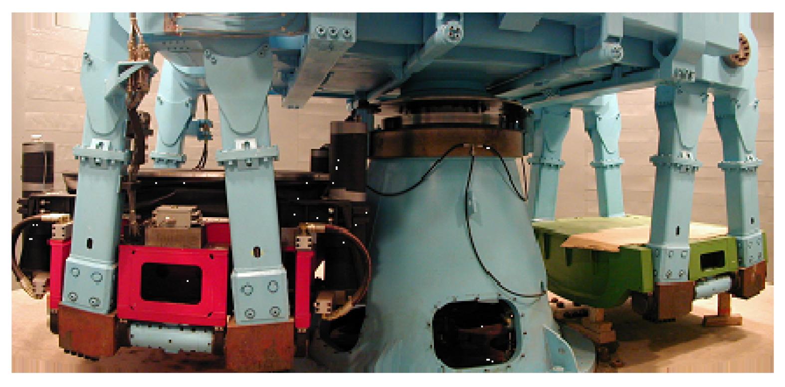
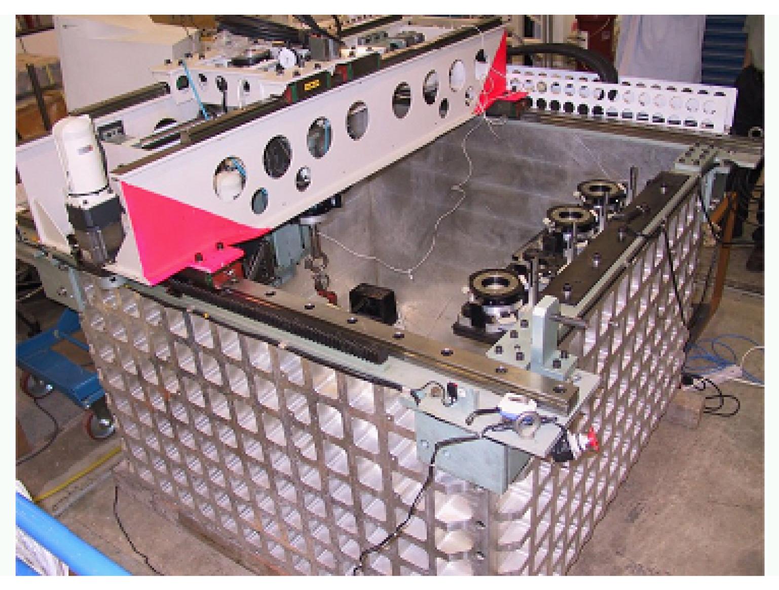
One of the most advanced geotechnical centrifuges in the world was established at HKUST in April 2001 (Ng et al., 2001a), as shown in Fig. 4. This 400g-t geotechnical centrifuge is equipped with advanced simulation capabilities including the world’s first in-flight bi-axial (2D) shaker, an advanced four-axis robotic manipulator and a state-of-the-art data acquisition and control system. Figs. 5 and 6 show the bi-axial shaking table (Shen et al., 1998; Ng et al., 2001a) and the four-axis robotic manipulator (Ng et al., 2002), respectively.
Fig.4 The 8.5 m-diameter (400g-t) beam centrifuge at HKUST
This 8.4 m diameter beam centrifuge is equipped with two swinging platforms, one for static tests and one for dynamic tests. For static tests, the centrifuge is able to accommodate a model size of up to 1.5 m×1.5 m×1 m. The centrifugal acceleration can be up to 150g. For dynamic tests, the centrifuge incorporates a unique bi-axial servo-hydraulic shaker (Fig. 5) to model earthquake-induced engineering problems (Ng et al., 2001a; 2004b). The bi-axial shaker is capable of simulating earthquake motions in two horizontal directions simultaneously. The shaker can accommodate a mode size of up to 0.6 m×0.6 m×0.4 m and up to 3000 N in weight. The centrifuge can be operated at up to 75g for dynamic tests.
Fig.5 The bi-axial shaking table at HKUST
As shown in Fig. 6, the advanced and state-of-the-art four-axis robotic manipulator has incorporated a tool changer and four tool adopters to permit interchanging tools without stopping the centrifuge. At a centrifugal acceleration of 100g, the robotic manipulator can produce a torque up to ±5 MN·m and prototype loads of ±10 MN, ±10 MN, and 50 MN forces in the x, y, and z directions, respectively.
Fig.6 The four-axis robotic manipulator at HKUST
Fig. 7 compares the capacity of major geotechnical centrifuges worldwide. Acronyms of some institutions in the figure are given in Appendix.
Fig.7 Capacity of the major geotechnical centrifuges in the world
It can be seen that the capacity of the centrifuge at HKUST (400g-t) is one of the largest in the world. This centrifuge has been used to model and investigate various complex and challenging geotechnical problems. Four examples are reported and interpreted in the following sections.
6.1. Example 1: correction of building tilt by in-flight soil extraction
6.1.1. Introduction
Building tilt is frequently encountered where ground is not homogeneous or there are adjacent underground constructions conducted. To correct building tilts, some solutions have been proposed. The Italian engineer Terracina (1962) proposed one possible way to correct the Leaning Tower of Pisa, by extracting soil through inclined boreholes from the less settled side of the leaning tower. Similar to soil extraction through inclined boreholes, the use of relief boring techniques with soil extraction through vertical boreholes is popular in China to reduce tilting and to stabilise buildings on soft ground. It is recognised that vertical soil extraction is generally simpler than an inclined extraction underneath the foundation of a tilted building. However, the effectiveness of vertical boring, as compared with inclined drilling, is somewhat doubtful and is questioned by some engineers. Sometimes the design of remedial action to reduce building tilt is essentially empirical. To investigate the effectiveness of vertical soil extraction, in-flight vertical boring adjacent to an initially tilted building was simulated, by the four-axis robotic manipulator at HKUST. In addition, results of the centrifuge test were compared with predictions from a theoretical elastic solution based on Mindlin (1936)’s equations (Ng and Xu, 2003).
6.1.2. Test setup, model preparation, and procedure
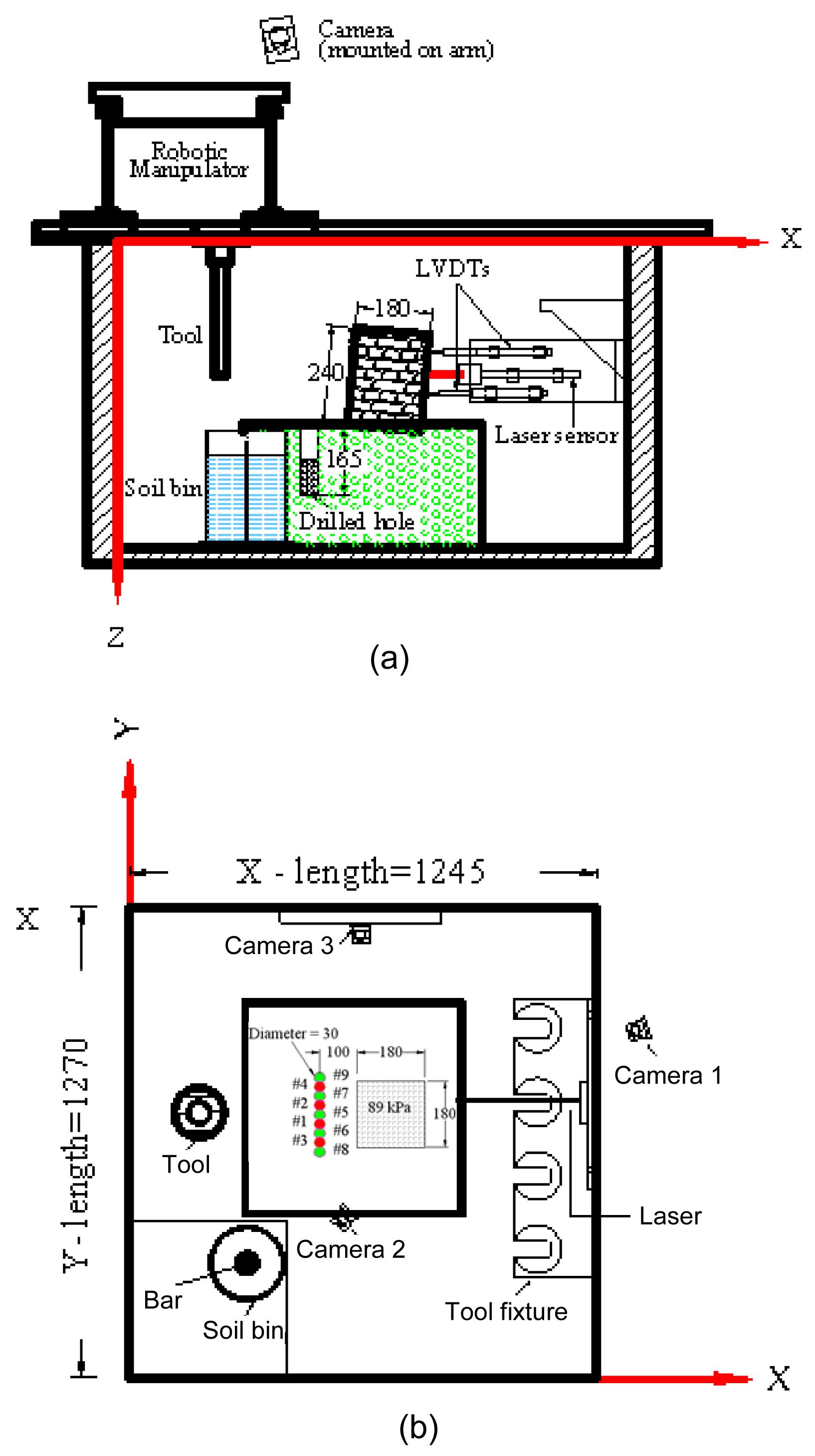
Fig. 8 shows the test setup as reported by Ng and Xu (2003).
Fig.8 Centrifuge test setup: (a) elevation view; (b) plan view (all dimensions in mm, unless stated otherwise)
The test was conducted at 30g. The simulated building had a 5.4 m×5.4 m base area (in prototype) and was approximately nine-storeys tall (in prototype), which generated an average bearing pressure of 89 kPa on the ground. The model ground consisted of an unsaturated completely decomposed granite (CDG) prepared at an average initial water content of 15.3% and a dry unit weight of 13.0 kN/m3. A hollow cylinder extracting tool with an external diameter of 30 mm and a soil bin were developed for the test. The movements of the building were measured by two linear variable differential transformers (LVDTs) and one non-contact laser displacement transducer. The performance of the robot and the model was monitored by five cameras at different locations.
When the centrifuge was spun up to 30g, the building was at an initial tilt of 1/27. To correct the tilted building, some soil was extracted from the ground in the opposite side of the tilt by drilling two series of holes. The sequence of drilling hole is shown in Fig. 8b. The holes were 160 mm deep and 100 mm away from the building. Each hole was drilled in two steps, each 80 mm in depth. Converted to prototype scale, each hole was 0.9 m in diameter and 4.8 m deep, and was 3 m away from the building.
6.1.3. Effects of soil extraction on building tilt
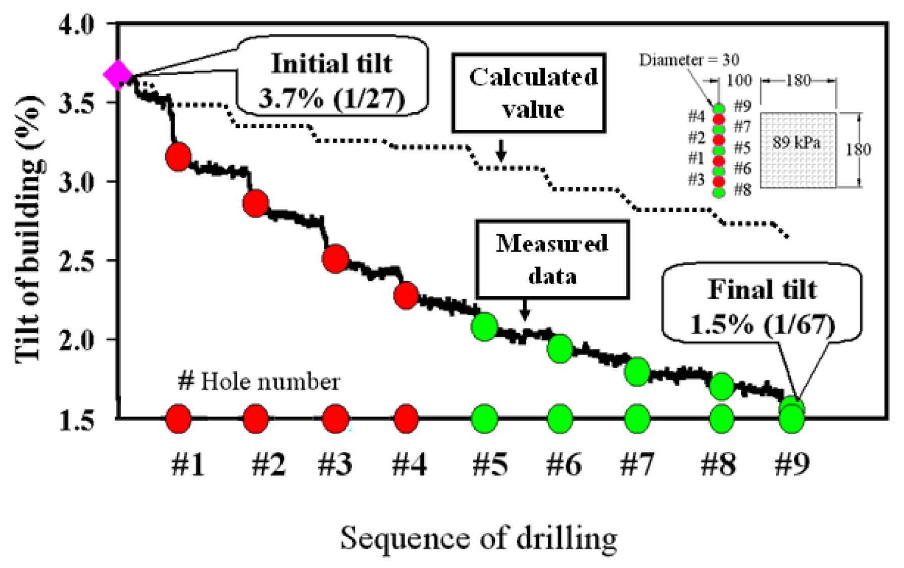
Fig. 9 shows the development of building tilt during soil extraction. The building tilt calculated by a theoretical elastic solution is also included for comparison (Ng and Xu, 2003). The measured results show that drilling of the first series of holes (holes #1–4) caused a 1.5% reduction of the building tilt while the second series of holes (holes #5–9) caused a further 0.7% correction to the building.
Fig.9 Development of tilting of model building during soil extraction (all dimensions in mm, unless stated otherwise)
After drilling nine holes, the final tilt of the building was reduced to 1.5%. This test clearly demonstrated the effectiveness of correcting building tilt by vertical soil extraction.
Based on Mindlin (1936)’s equation, Ng and Xu (2003) derived an elastic solution and compared it with the centrifuge test results by soil extraction. As expected, the calculated change of building tilt (Fig. 9) shows a similar trend to the measured building tilt, but with a much smaller magnitude (only 45% of the measured value at the final stage). Two major reasons for the underestimation are:
(1) The solution is derived for vertical boring of a single hole, so the influence of a previous boring on a subsequent one was not taken into account.
(2) Yielding and plastic deformation of the soil were not considered.
Therefore, the construction sequence and the plastic deformation of soil should be taken into account when predicting the correction of building tilt.
6.2. Example 2: effects of collapse of a tunnel on an existing tunnel
6.2.1. Introduction
Rapid development in urban areas leads to a high demand for transportation of people and vehicles. Tunnels are often constructed to reduce congestion and to serve as vital conduits for the movement of vehicles. Sometimes, it is inevitable that multiple tunnels are constructed very close together due to intensive use of underground space (Ng et al., 2004a). Tunnel excavation will result in volume loss which induces movement and stress change in the soil around adjacent tunnels. An extreme case of tunnel-tunnel interaction problem would be the influence of a tunnel collapse on an adjacent tunnel. One typical example is the collapse of the Heathrow Express Tunnel in 1994 when the collapse of three tunnels occurred during the construction of a new tunnel in London Clay (HSE, 2000). Therefore, an understanding of the effects of multiple tunnel interaction is essential to develop an improved design guide so that precautions can be taken during and after new tunnel construction. The effect of tunnel collapse on a nearby existing tunnel has been investigated by carrying out centrifuge tests (Ng et al., 2003).
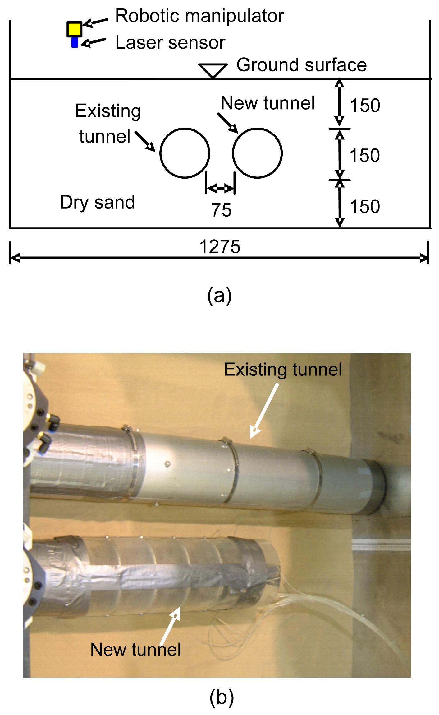
6.2.2. Centrifuge model package
Figs. 10a and 10b show elevation view and bird’s eye view of the model package, respectively (Ng et al., 2003). The test was carried out at 60g. The existing model tunnel was made of an aluminium-alloy pipe with an external diameter of 150 mm, wall thickness of 3.3 mm, and longitudinal length of 1243 mm. The estimated EI in transverse section per metre run was 0.21 kN·m2, which was used to represent a prototype reinforced concrete tunnel of an external diameter of 9 m, wall thickness of 0.268 m, and a length of 74.6 m. The new tunnel with prototype diameter of 9 m and length of 27 m was designed to simulate an open-face excavation similar to an idealised New Austrian Tunnelling Method (NATM). The idealised NATM was simulated by using 12 semi-circular airbags, i.e., 12 compartments (Fig. 11). Each semi-circular airbag was 150 mm in diameter and separated by 3 mm thick aluminium-alloy dividers. Each pair of semi-circular airbags was used to mimic the left drift and right drift of a NATM tunnel. The advance of the new tunnel was simulated by reducing the air pressure inside the airbags at the construction stages indicated in Fig. 11.
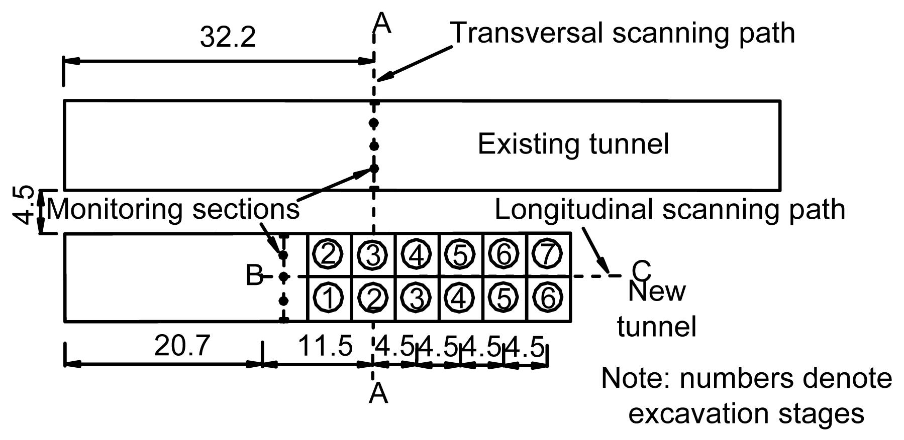
Fig.11 Layout of tunnels and monitoring sections (unit: m)
Dry Leighton Buzzard (LB) sand fraction E was used in the test. The maximum and minimum unit weight of the sand was equal to 15.9 kN/m3 and 13.2 kN/m3, respectively. In this centrifuge test, the unit weight of the sand was 14.2 kN/m3 (i.e., relative density=50%).
6.2.3. Instrumentation and testing procedure
Fig. 11 shows the plan view of the twin tunnels and two monitoring sections in prototype scale (Ng et al., 2003). In each monitoring section, eight miniature pressure cells and eight pairs of strain gauges were installed evenly with an interval of 45° around the circumference of each tunnel. The pressure cells were mounted on the outer surfaces and the strain gauges were glued onto both the outer and inner surfaces of the tunnels to measure circumferential distributions of axial strain and bending strain. Three-dimensional ground surface profiles were measured by using a laser sensor mounted on the robotic manipulator in-flight (Fig. 10a). Two travelling and scanning paths along sections AA and BC by the robotic manipulator were adopted and controlled by a computer.
During the swing-up of the centrifuge, the air pressure inside the airbags was increased to balance the increased overburden pressure as the centripetal acceleration was increased. When the centripetal acceleration reached 60g, the construction of the new tunnel was started by depressurising the airbags in different stages to stimulate an idealised NATM. The construction sequence was divided into seven stages starting from the right drift of the tunnel, as indicated by the stage numbers shown in Fig. 11.
6.2.4. Three-dimensional ground surface settlements and bending moments
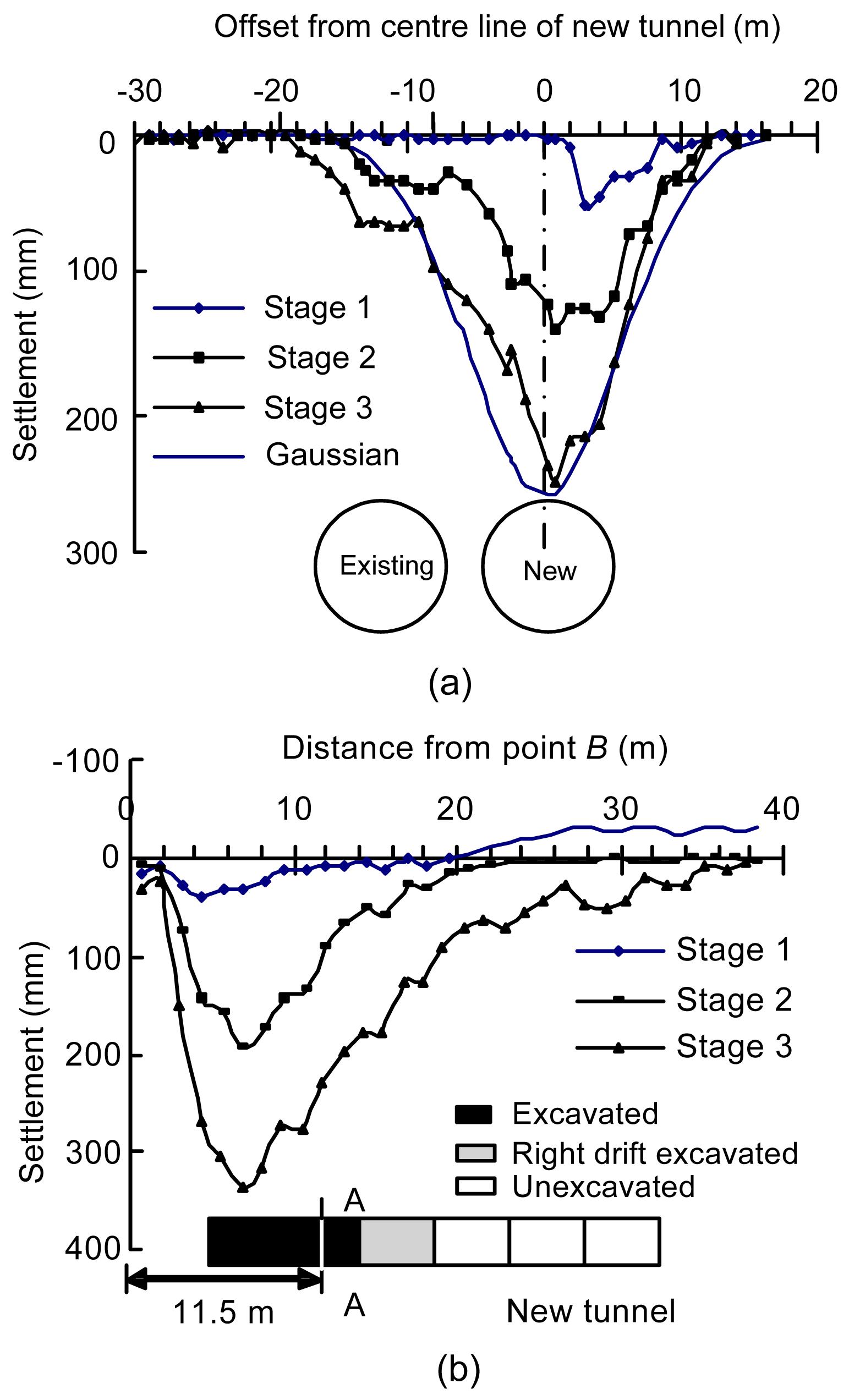
Figs. 12a and 12b show the measured settlements along the transverse path AA and the longitudinal path BC from excavation stage 1 to stage 3, respectively. The results are presented in prototype scale unless stated otherwise.
Fig.12 Three-dimensional settlement bowl along transverse direction (a) and longitudinal direction (b) of the new tunnel
After excavation stage 1, a settlement trough formed at section AA with the maximum settlement above the right drift of the tunnel, as expected. As the tunnel advanced, the transverse settlement trough at the section became deeper and wider with the location of the maximum settlement shifted towards the centreline of the tunnel. By fitting a Gaussian distribution with the maximum settlement of 260 mm and the point of inflection of the settlement trough equal to 5.5 m, it can be seen that there was a considerable discrepancy between the fitted distribution and the measured settlements above the left drift of the tunnel, possibly attributable to the presence of the existing tunnel and the excavation sequence adopted. In the longitudinal direction, the measured settlements increased with the advance of the tunnel as expected and the measured maximum settlements were consistent with those along the transverse section and a 3D settlement bowl can be deduced.
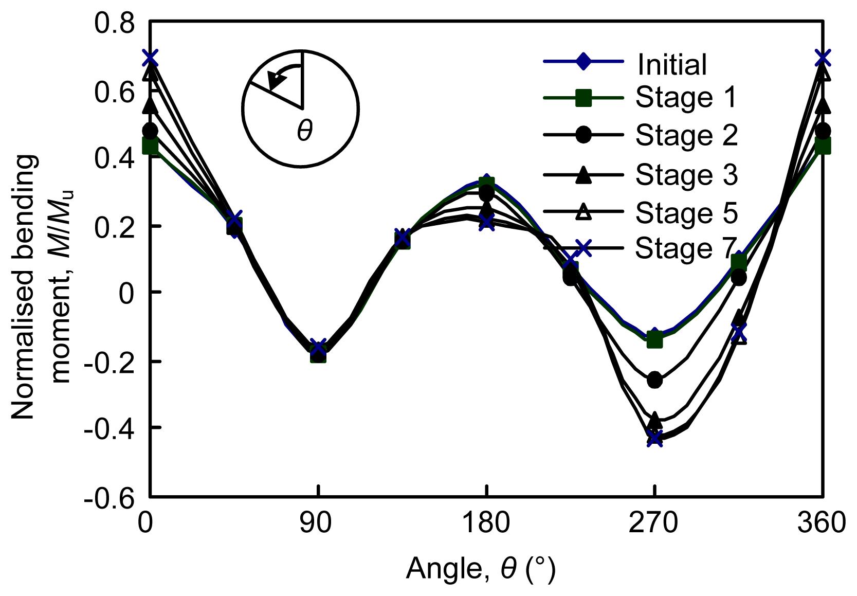
Fig. 13 shows the measured bending moments (BM) normalised by the ultimate moment capacity, Mu. For the model tunnel with an estimated yield stress of 100 MPa, the calculated ultimate moment capacity was Mu=0.272 kN·m/m. The maximum positive BM was induced at the crown (θ=0°) and at the invert (θ=180°) of the existing tunnel. As expected, the BM increased as the tunnel advanced, particularly at the crown. On the other hand, the maximum normalised negative BM occurred at the left and the right springlines (i.e., θ=90° and θ=270°, respectively). The BM at θ=270° increased steadily whereas the BM at θ=90° remained almost unchanged. Based on the measurements, it can be deduced that the tunnel deformed into an elliptical shape. The absolute increase in BM due to tunnelling was 60%, 28%, and 228% at the crown, invert, and the right springline of the existing tunnel, respectively.
Fig.13 Normalised bending moment distribution
Recently, Ng et al., (2013a) have also reported a series of 3D centrifuge tests investigating the responses of an existing tunnel to the excavation of a new tunnel perpendicularly underneath it. 3D tunnel advancement was simulated using a novel technique that considers the effects of both volume and weight losses in-flight. This novel technique involves using a “donut” to control volume loss and mimic soil removal in-flight. To improve fundamental understanding of stress transfer mechanism, measured results were back analyzed three-dimensionally using the finite element method using an advanced soil model, which can capture soil behaviour at small strains. It is found that the maximum measured settlement of the existing tunnel induced by the new tunnel constructed underneath was about 0.3% of tunnel diameter, which may be large enough to cause serviceability problems. The observed large settlement of the existing tunnel was caused not only by a sharp reduction in vertical stress at the invert but also by substantial overburden stress transfer at the crown. The section of the existing tunnel directly above the new tunnel was vertically compressed because the incremental normal stress on the existing tunnel was larger in the vertical direction than in the horizontal direction. The tensile strain and shear stress induced in the existing tunnel exceeded the cracking tensile strain and allowable shear stress limit given by the American Concrete Institute.
6.3. Example 3: excavation effects on pile capacity
6.3.1. Introduction
Conventionally, pile loading tests are carried out at the ground surface, prior to a basement excavation. A sleeve is often used in the loading test to eliminate shaft resistance within the depth of future excavation, in order to predict the behaviour of the piles working underneath the basement. Following such a test procedure, the stress changes in the soil due to excavation are not captured. Predicting the performance of piles beneath a basement from the conventional loading tests may pose a challenge for engineers.
In order to study the influence of excavation on pile capacity, centrifuge modelling of single pile loading tests was carried out in dry Toyoura sand (Zheng et al., 2010; 2012). In-flight pile loading tests were carried out both at the ground surface prior to excavation and at the formation level after excavation. Model piles with two distinct interfaces (i.e., low friction and high friction) were also simulated to investigate the influence of interface roughness on pile behaviour and capacity.
6.3.2. Model setup and testing procedures
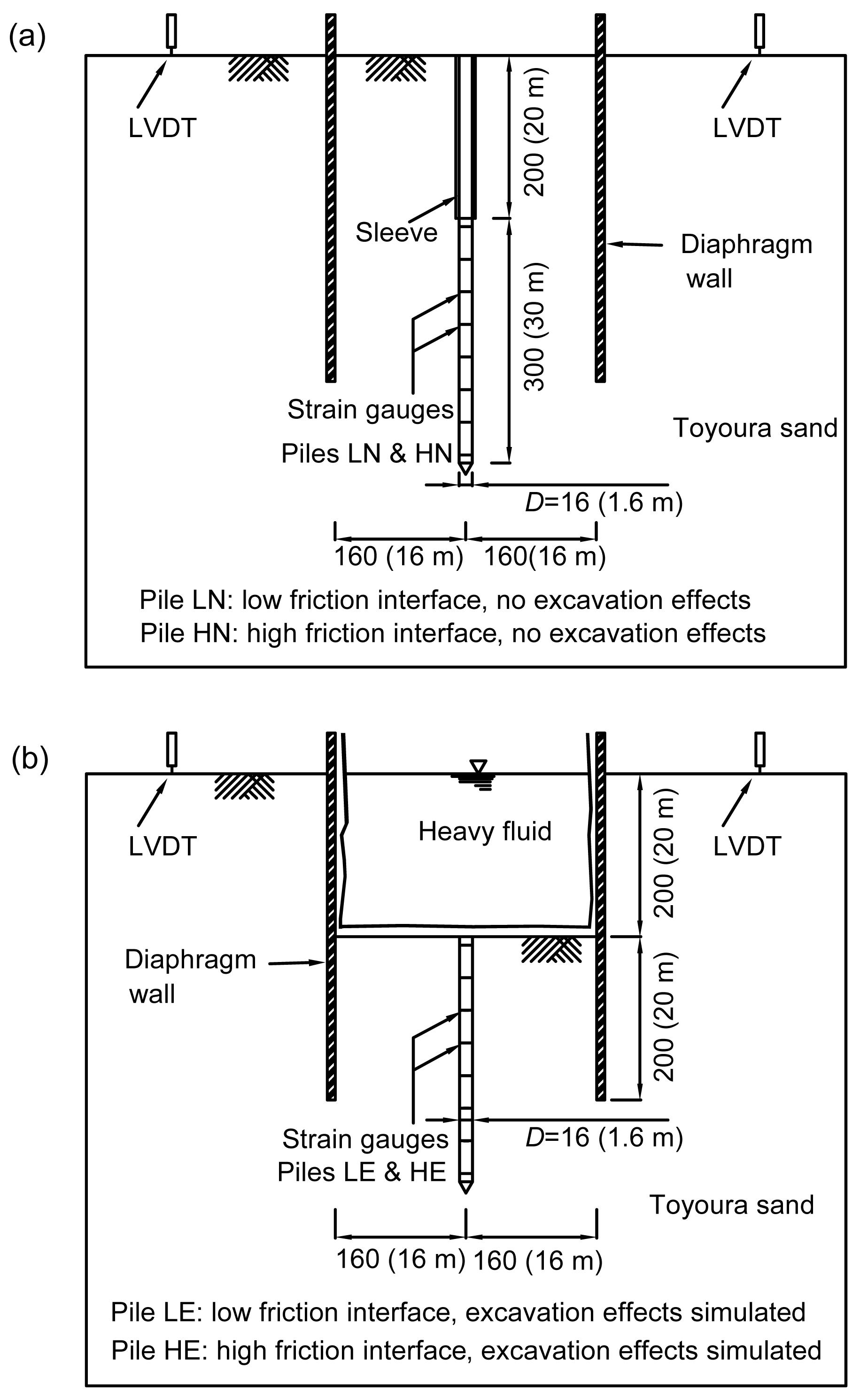
Fig. 14a shows a schematic diagram of the tests which are intended to model conventional pile loading tests. In-flight loading tests were carried out at the ground surface. A sleeve was used for the upper portion of the pile to eliminate shaft resistance within the depth of future excavation. Fig. 14b shows the tests which are intended to model pile loading tests carried out after excavation.
Fig.14 Schematic diagrams of the centrifuge models: (a) piles tested at ground surface (LN and HN); (b) piles tested after excavation (LE and HE) (Units: mm. Numbers in parenthesis denote corresponding prototypes)
In-flight basement excavation was simulated by draining away zinc chloride solution, which had the same density as that of the sand. A circular model diaphragm wall was used to retain the excavation. The lateral stiffness of the diaphragm wall was very large, and hence the lateral deformation caused by the excavation was negligible. After excavation, an in-flight pile loading test was carried out at the basement level. In each of the tests, an instrumented single pile was located at the centre of the excavation area. All the centrifuge tests were performed at 100g.
Model piles with two distinct interfaces were used. They were defined as “low friction piles” and “high friction piles” (Zheng et al., 2012). Normalised roughness Rn (Kishida and Uesugi, 1987) of the two interfaces were 0.018 and 0.21, respectively. According to laboratory tests (Kishida and Uesugi, 1987; DeJong and Frost, 2002; Fioravante, 2002), for the low friction piles under loading, particle sliding failure happens at the soil-pile interface. These low friction piles are therefore intended to simulate piles in non-dilatant geo-materials (such as normally consolidated clay and loose sand). In contrast, for the high friction piles, failure happens within the soil surrounding the piles. Volume change takes place in the shear band according to the density and the stress level of the soil. The high friction piles are therefore intended to simulate piles in dilatant geo-materials (such as dense sand).
The pluvial deposition method was used to rain sand into the model container from a hopper. After the formation of sand bed, the model pile was temporarily fixed in its designed location. Then the process of sand raining was continued. By using the pluvial deposition method to form sand bed around the pile at 1g, the initial stress around the model pile is small. Subsequently, as the g-level increased during a test, the initial stress around the pile also increased under the Ko conditions, which could be regarded as similar to that adjacent to a non-displacement pile. The measured average relative densities of the sand in the four tests ranged from 58% to 64%, with an average value of 62%.
All the test results are converted to prototype scale unless stated otherwise.
6.3.3. Influence of excavation on pile performance and capacity
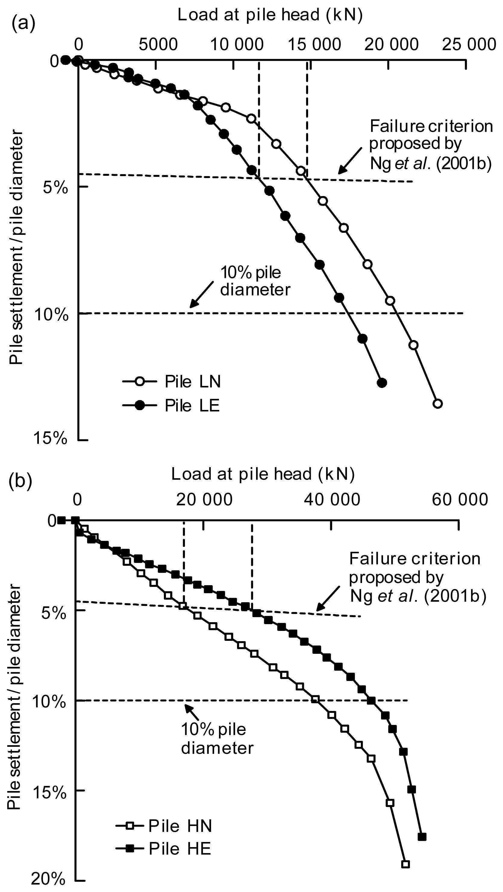
Fig. 15a shows the normalised load-settlement relationships of the low friction piles. To compare the ultimate pile capacities, the failure criterion proposed by Ng et al. (2001b) is used. This is a semi-empirical method for the interpretation of a moderately conservative failure load. The criterion for floating piles is given by
,
where ΔM
is the maximum pile head movement to define the ultimate load; D is the pile diameter; P is the applied test load; L is the pile length; A is the pile shaft cross-sectional area; and E is the pile shaft modulus of elasticity.
Fig.15 Load-settlement curves: low friction piles (LN and LE) (a); high friction piles (HN and HE) (b)
As shown in the figure, the interpreted capacities of the two 1.6 m-diameter piles (LN and LE) are 14 700 kN and 11600 kN, respectively. The capacity of pile LE is 80% of that of pile LN. For comparison, the failure criterion based on a pile settlement of 10%D is also illustrated in the figure. If this criterion is adopted, the capacity of pile LE is 84% of that of pile LN. It is evident that the capacity of a low friction pile is reduced by 16%–20% after excavation due to the vertical stress relief.
Fig. 15b shows the load-settlement relationships of the high friction piles (Zheng et al., 2012). As an incremental load is applied, the pile tested after excavation (HE) has slightly higher stiffness than that of pile HN. Using the same failure criterion (Ng et al., 2001b), interpreted capacities for piles HN and HE are 16 960 kN and 27 680 kN, respectively. The capacity of pile HE is 39% higher than that of pile HN. Based on these results, the capacity of a high friction pile is increased after excavation. This finding is opposite to the results for the low friction piles. The increase in pile capacity after excavation is probably attributable to the increase in horizontal stress resulting from strong soil dilation at the high friction pile-soil interface.
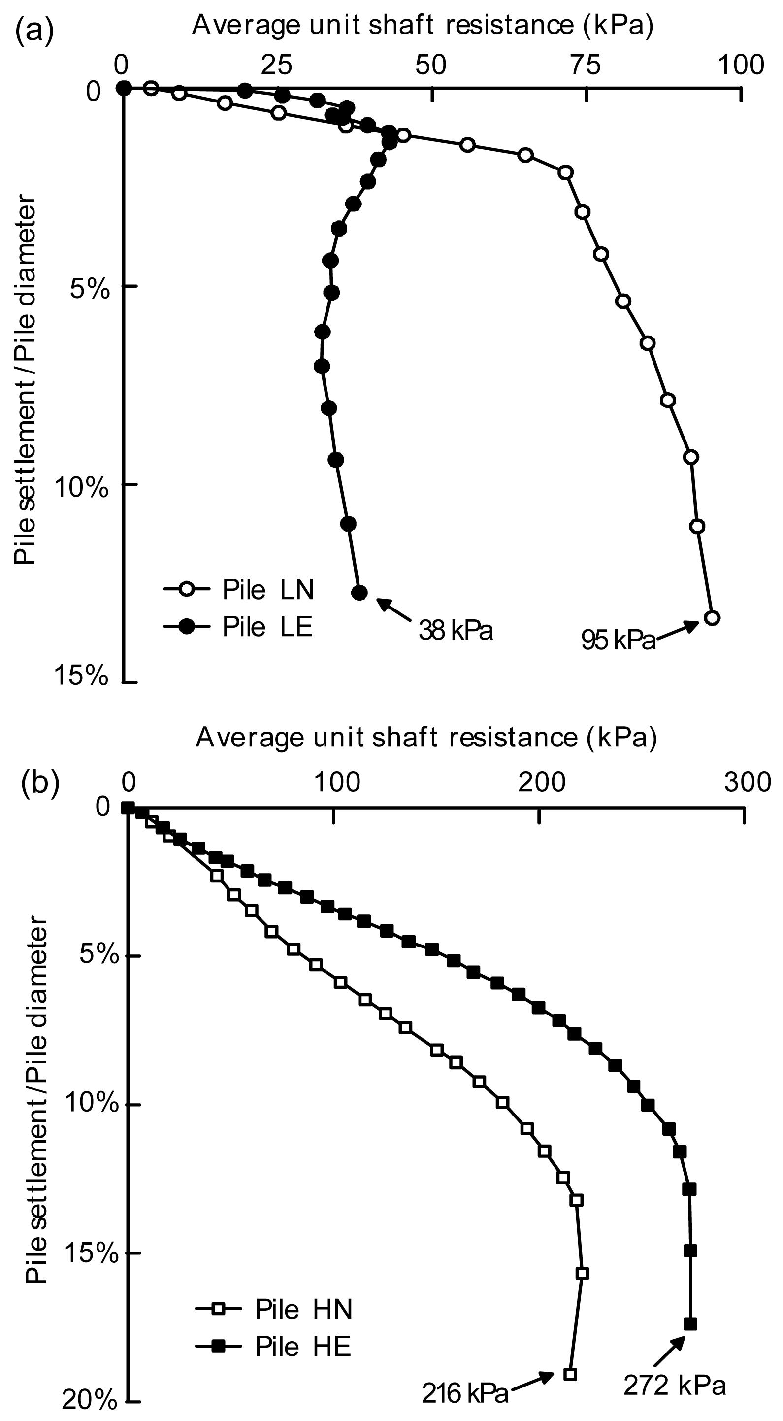
Fig. 16a shows the mobilisation of the average unit shaft resistance for the low friction piles (Zheng et al., 2010). The shaft resistance of each pile is calculated by subtracting the toe resistance from the total load applied at the pile head. At the final loading stage, the average unit shaft resistance of pile LN is 95 kPa. In contrast, the unit shaft resistance of pile LE is only 38 kPa, which is 40% of that of pile LN. The reduction in the unit shaft resistance is closely related to the change in the effective stress level for the two cases. It is found that the ultimate unit shaft resistance of a low friction pile decreases in proportion to the effective stress relief resulting from excavation.
Fig.16 Average unit shaft resistances: low friction piles (LN and LE) (a); high friction piles (HN and HE) (Zheng et al., 2012) (b)
Fig. 16b shows the average unit shaft resistance for the high friction piles (Zheng et al., 2012). At the final loading stage, the average unit shaft resistance of pile HE is about 272 kPa, which is 26% higher than that of pile HN (216 kPa). This result is consistent with the higher capacity of pile HE, as shown in Fig. 16b. This measured increase in unit shaft resistance may be due to the increase in horizontal stress resulting from the dilative behaviour of the soil-pile interface.
Recently Ng et al. (2013b) have also reported two 3D centrifuge tests investigating the effects of a basement excavation on an existing tunnel. In addition, a preliminary 3D numerical analysis was conducted to back-analyse the centrifuge tests and to study the effects of the tunnel cover-to-diameter and unloading ratios on the existing tunnel. For the specific conditions simulated and soil type tested, a maximum heave of about 0.07% of the final depth of the basement excavation (He) was induced in the tunnel that ran parallel to and beneath the basement. On the contrary, a maximum settlement of 0.014% He was induced in the tunnel located at the side of the basement. For the former tunnel, the influence zone by the basement excavation on vertical tunnel displacement along the longitudinal direction was 1.2L (basement length). By studying the measured strains in the longitudinal direction of the existing tunnel, it was found that the inflection point, where the shear force is at a maximum, was located at 0.8L away from the basement centre. Due to stress relief from the basement excavation, the tunnel that located directly beneath the basement was vertically elongated but the one that lay at the side of the basement was distorted. A preliminary numerical parametric study found that tunnel heave decreased as the cover-to-diameter ratio increased but at a reduced rate.
6.4. Example 4: liquefied flow and non-liquefied slide of loose fill slopes
6.4.1. Introduction
Slope failures occur in many parts of the world. A slope will become unstable when its shear resistance is smaller than any external driving shear stress, which may be induced by mechanical and hydraulic means such as rainfall, earthquake, vibration, and seepage. Alternatively, a slope will also become unstable if its shear resistance has deteriorated and reduced due to weathering and any other mechanisms such as static liquefaction. Very often the terminology “static liquefaction” is used to describe soil slope failures and is reported in the literature. However, it is evident that different researchers and engineers are referring to different failure mechanisms. Some use debris mobility (travel angle or run out distance) to judge whether a slope failure has been caused by liquefaction or not. Clearly there is no direct relationship between liquefaction and mobility. For instance, level ground can liquefy (at zero/small effective stress under seismic loading) with zero run out distance. On the contrary, a steel ball can run down a bare slope and travel a long way but that has nothing to do with liquefaction (Ng, 2009).
What is static liquefaction? How is it triggered? What is the effective stress at failure, if the slope is fully saturated initially, as in an undersea slope? How can we identify and define static liquefaction failures? Does a strain-softening material necessarily mean static liquefaction? Is there any difference between slide failure and flow failure? What is the role of hydrofracture? How does the angle of a slope affect the so-called static liquefaction? Is there any difference between fluidisation and liquefaction? Will static liquefaction occur in unsaturated soil slopes? How does the angle of a slope affect the potential of static liquefaction? Is there any relationship between the so-called static liquefaction failure and run out distance? Can soil nails be used to stabilise any loose fill slopes? Some of these questions have not been well understood and addressed and some of them may be even controversial. Some selected issues discussed above were investigated by Ng (2005; 2007; 2008) by means of laboratory triaxial element tests and centrifuge model tests on loose fill slopes using gap-graded LB sand and a well-graded silty sand (i.e., CDG). Observed key failure mechanisms of static liquefaction in the LB sand and non-liquefied slides of CDG fill slopes are identified and discussed.
6.4.2. Clarification of some terminologies relating to static liquefaction
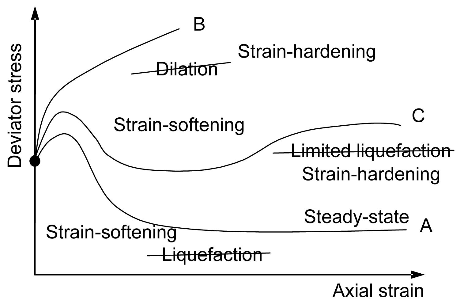
Fig. 17 shows some typical results from undrained monotonic loading triaxial tests on saturated, anisotropically consolidated sand specimens. As illustrated, a very loose sand specimen, A, exhibits a peak undrained shear strength at a relatively small shear strain and then “collapses” to much smaller shear strength at large strains. This behaviour is often casually referred to as “liquefaction” or “flow liquefaction” by many researchers and engineers. No matter whether it is called “flow liquefaction” or “liquefaction”, the terminology used to describe the behaviour observed in the laboratory is rather confusing and, strictly speaking, incorrect. Would it be clearer and more precise to describe the material behaviour of the loose specimen, A, and a dense specimen, B, as “strain-softening” and “strain-hardening”, respectively? It must be pointed out that these are just the behaviour of the material element and do not necessarily capture and represent the global behaviour of an entire fill slope or an earth structure.
Fig.17 Incorrect interpretations of liquefaction, limit liquefaction and dilation in undrained monotonic loading tests on sand (modified from Castro (1969) and Kramer (1996))
6.4.3. Failure mechanism of liquefied flow in sand fill slopes
Slope centrifuge model tests were carried out to investigate the failure mechanisms of static liquefaction of loose fill slopes subjected to a rising ground water table (Zhang et al., 2006; Ng, 2009). LB Fraction E fine sand was selected as the fill material for the model tests, because of its pronounced strain-softening characteristics and its high liquefaction potential, i.e., a substantial reduction in shear strength when it is subjected to undrained shearing (Cai, 2001; Zhang, 2006). Fig. 18 shows the gap-graded particle size distribution of LB sand. D10 and D50 of the sand were 125 m and 150 m, respectively. Following BS1377 (1990), the maximum and minimum void ratios of the LB sand were found to be 1.008 and 0.667, respectively (Cai, 2001). The estimated saturated coefficient of permeability was 1.6×10⁻⁴ m/s.
Fig.18 Particle size distributions of LB sand and CDG
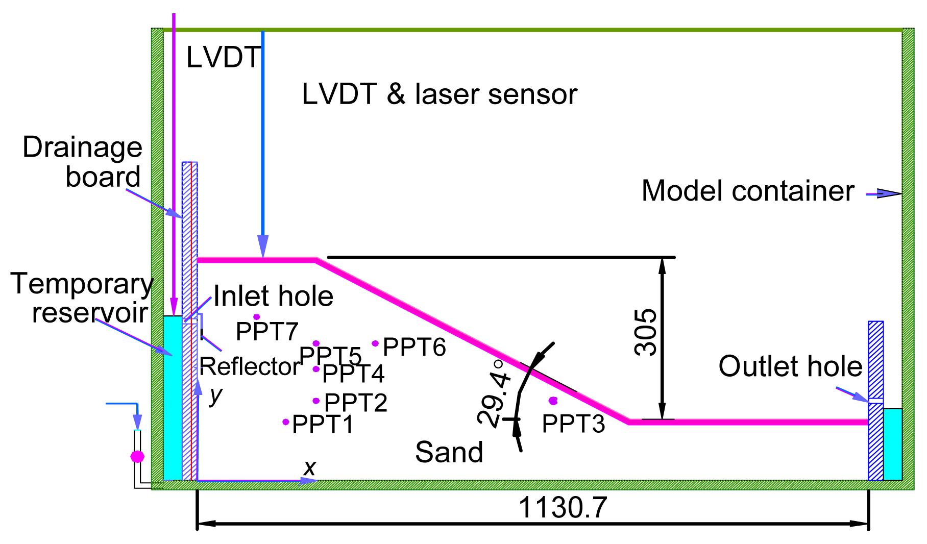
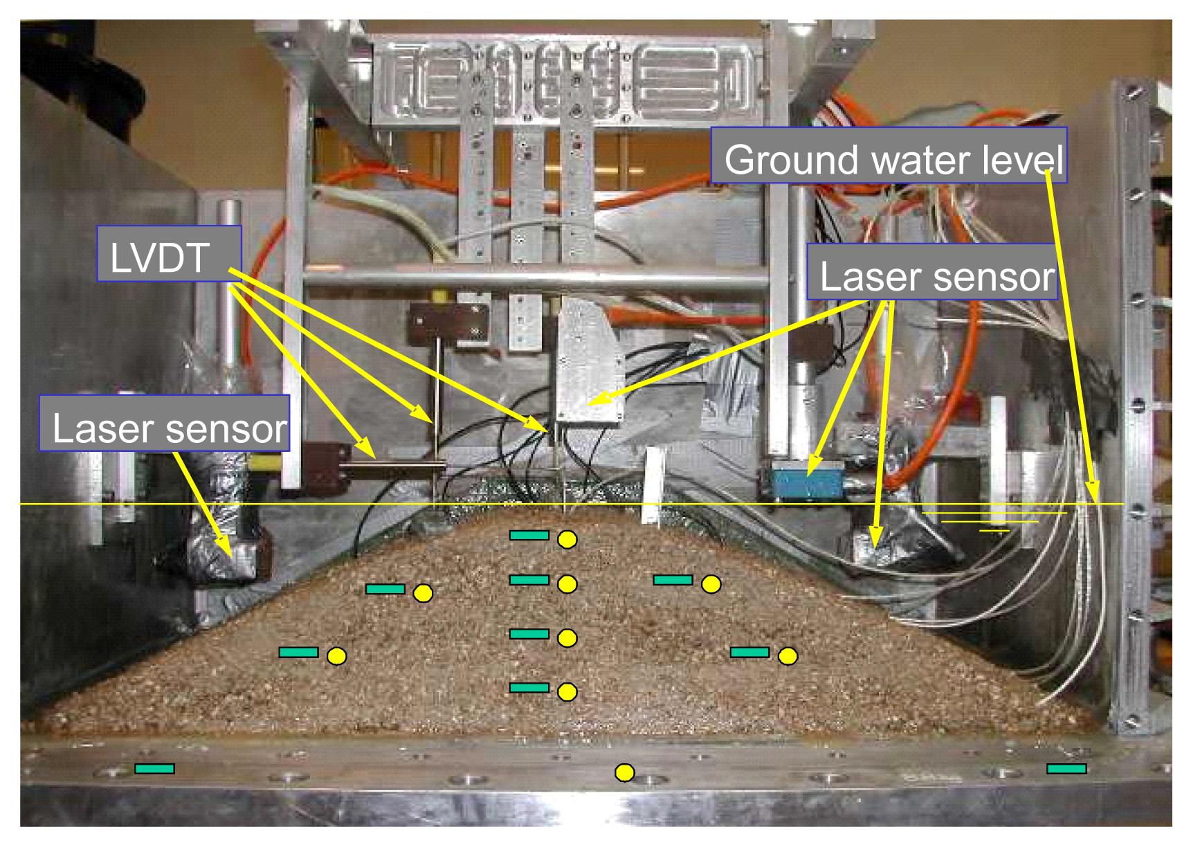
Fig. 19 shows an instrumented 29.4° loose sand fill slope model together with the locations of the pore water pressure transducers (PPTs) (Zhang and Ng, 2003; Ng, 2008). The model slope was prepared by moist tamping. The initial relative compaction was 68%.
Fig.19 Centrifuge model of a loose sand fill slope subjected to rising ground water table at 60g (unit: mm) (Zhang and Ng, 2003)
The body of the sand slope was instrumented with seven PPTs and arrays of surface markers were installed for image analysis of soil movements. LVDTs and a laser sensor were mounted at the crest of the slope to monitor its settlement.
Although the initial angle of the loose slope was prepared at 29.4° at 1g, the slope was densified to 80% of the maximum relative compaction due to self-weight compaction at 60g. The slope angle was therefore flattened to 24° (Fig. 20a), which is steeper than the angle of instability of 18.6°. This implies that the slope was vulnerable to instability, which could lead to liquefaction. At 60g, the 18 m-height (prototype) slope was destabilised by rising ground water from the bottom of the model (Zhang, 2006). The flow rate of the raising ground water was 9.6 mm/h in the model scale, corresponding to 573 mm/h in the prototype (based on a scaling factor of n for pore fluid velocity, Table 1).
Fig.20 Slope profile in a loose sand fill test before rising ground water table (a) and after static liquefaction (b) (Zhang and Ng, 2003; Ng et al., 2007)
The loose sand slope liquefied statically and flowed rapidly (Fig. 20b), i.e., it followed a process in which the loose slope was sheared under undrained conditions, lost its undrained shear strength as a result of the induced high pore water pressure and then flowed like a liquid, called “liquefied flow”.
Fig. 21 shows the measured rapid increase in the excess pore water pressure ratio (Δu/σ′v) within about 25 s (prototype) at failure at a number of locations in the slope during the test. The maximum measured Δu/σ′v was about 0.6, which would be much higher if a properly scaled viscous pore fluid were used to reduce the rate of dissipation of excess pore pressure in the centrifuge. This means that the slope would liquefy much more easily. As shown in Fig. 20b, the completely liquefied slope inclines at about 4° to 7° to the horizontal after the test. The observed fluidisation from in-flight video cameras and the significant rise in excess pore water pressures during the test clearly demonstrated the static liquefaction of the loose sand fill slope. It should be noted that measurements of sudden and significant rise of excess pore water pressures are essential to “prove” or verify the occurrence of static liquefaction of loose fill slopes if no video recording is available. The liquefaction of the loose sand slope was believed to be initially triggered by seepage forces in the test. It is obvious that soil nails cannot be used to stabilise a loose sand fill slope which has a high liquefaction potential.
Fig.21 Measured sudden and substantial increases in excess pore water pressure at seven locations inside the slope (Zhang and Ng, 2003; Ng, 2009)
6.4.4. Non-liquefied slide of shallow CDG fill slopes
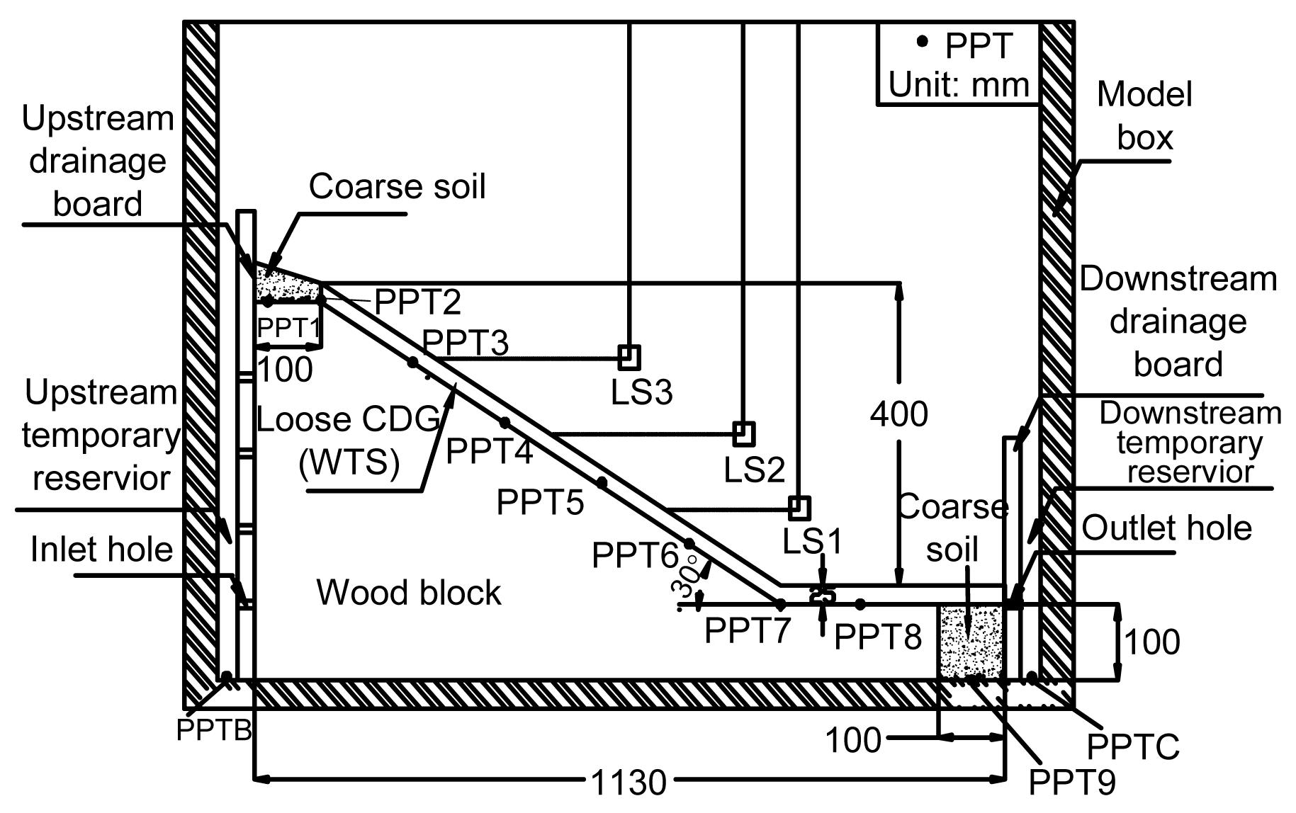
Apart from loose fill slopes using material with high liquefaction potential (i.e., LB), slopes loosely backfilled with a material with very small liquefaction potential (CDG) were also tested. Fig. 22 shows an instrumented centrifuge model for studying the potential static liquefaction of a loose shallow CDG fill slope subjected to a rising ground water table. The particle size distribution of the CDG used is denoted as WTS in Fig. 18. The initial fill density was 66%. This model was used to simulate a 1.5 m thick, 24 m high layered fill slope when tested at 60g. In addition to LSs installed for monitoring soil surface movements, PPTs were installed to measure excess pore water pressures during the tests. Effects of layering were considered by tilting the model container during model preparation. The slope was destabilised by downward seepage created by a hydraulic gradient, which was controlled by the water level inside the upstream temporary reservoir and the conditions of the outlet hole located downstream (Fig. 22). Two failures were induced in the test.
Fig.22 Model package of an instrumented shallow fill slope (Ng et al., 2007)
Figs. 23 and 24 show respectively the occurrence of a non-liquefied slide and the measured excess pore water pressure during two failures. The slide was initiated near the crest. Based on the observed failure mechanisms and the small excess pore water pressures measured, it was concluded that non-liquefied slide of loose shallow CDG fill slopes could occur but static liquefaction was very unlikely to happen. The significant difference between the observed centrifuge test results from the loose LB sand (Fig. 20b) and CDG fill slopes (Fig. 23) may be attributed to the difference in fine contents, gradation and liquefaction potential of the two materials.
Fig.23 Top view of the model showing a non-liquefied slide (Ng et al., 2007)
Fig.24 Variations in the measured pore water pressure at the crest (PPT2) and at the toe (PPT7) of the slope with time (Ng et al., 2007)
6.4.5. Response of loose CDG slopes to earthquakes
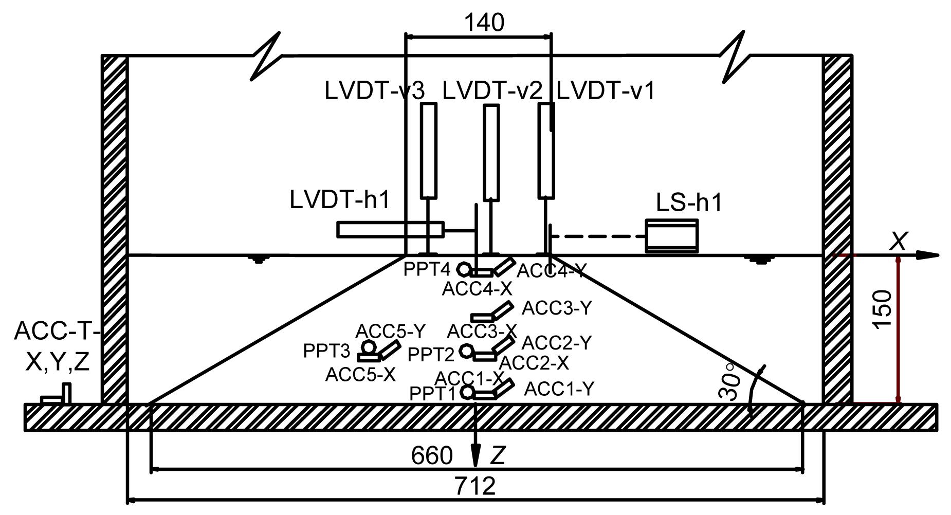
To further investigate the possibility of flow liquefaction of loose CDG fill slopes, uni-axial and bi-axial dynamic centrifuge tests were carried out (Ng et al., 2004b). The model CDG fill slopes were subjected to shaking ranging from 0.08g to 0.28g (prototype) in the centrifuge at HKUST. All the models were essentially the same in geometrical layout and made of loose CDG with the same initial dry density. Fig. 25 shows a typical model slope (6 m in prototype) initially inclined at 30° to the horizontal, with its instrumentation. A rigid rectangular model box was used to contain the CDG samples compacted to an initial dry density of about 1.4 g/cm3 (or 77% of relative compaction). Five pairs of miniature accelerometers (ACCs) were installed in the slope. Each pair was arranged to measure soil accelerations in two horizontal directions (i.e., X- and Y-direction). Four miniature PPTs were installed in the soil near the accelerometers to record pore water pressures during shaking. On top of the slope, three LVDTs were mounted to measure the crest settlement, and one LVDT and one LS were used to measure horizontal movement of the crest.
Fig.25 Configuration of the model slope and instrumentation (Ng et al., 2004b) (unit: mm)
To simulate the correct dissipation rate of excess pore pressures in the centrifuge tests, sodium carboxy methylcellulose (CMC) powder was mixed with distilled deionized water to form the properly scaled viscous pore fluid and to saturate the loose CDG model slopes.
After model preparation, the speed of the centrifuge was increased to 38g. Once a steady state pore pressure condition was reached at all transducers, a windowed 50 Hz (1.3 Hz prototype), 0.5 s (19 s prototype) duration sinusoidal waveform was then applied (Ng et al., 2004b). After triggering each earthquake, the centrifuge acceleration was maintained long enough to allow the dissipation of any excess pore pressure. This paper only highlights some important results from one biaxial shaking test. Other details of all the tests were presented in (Ng et al., 2004b).
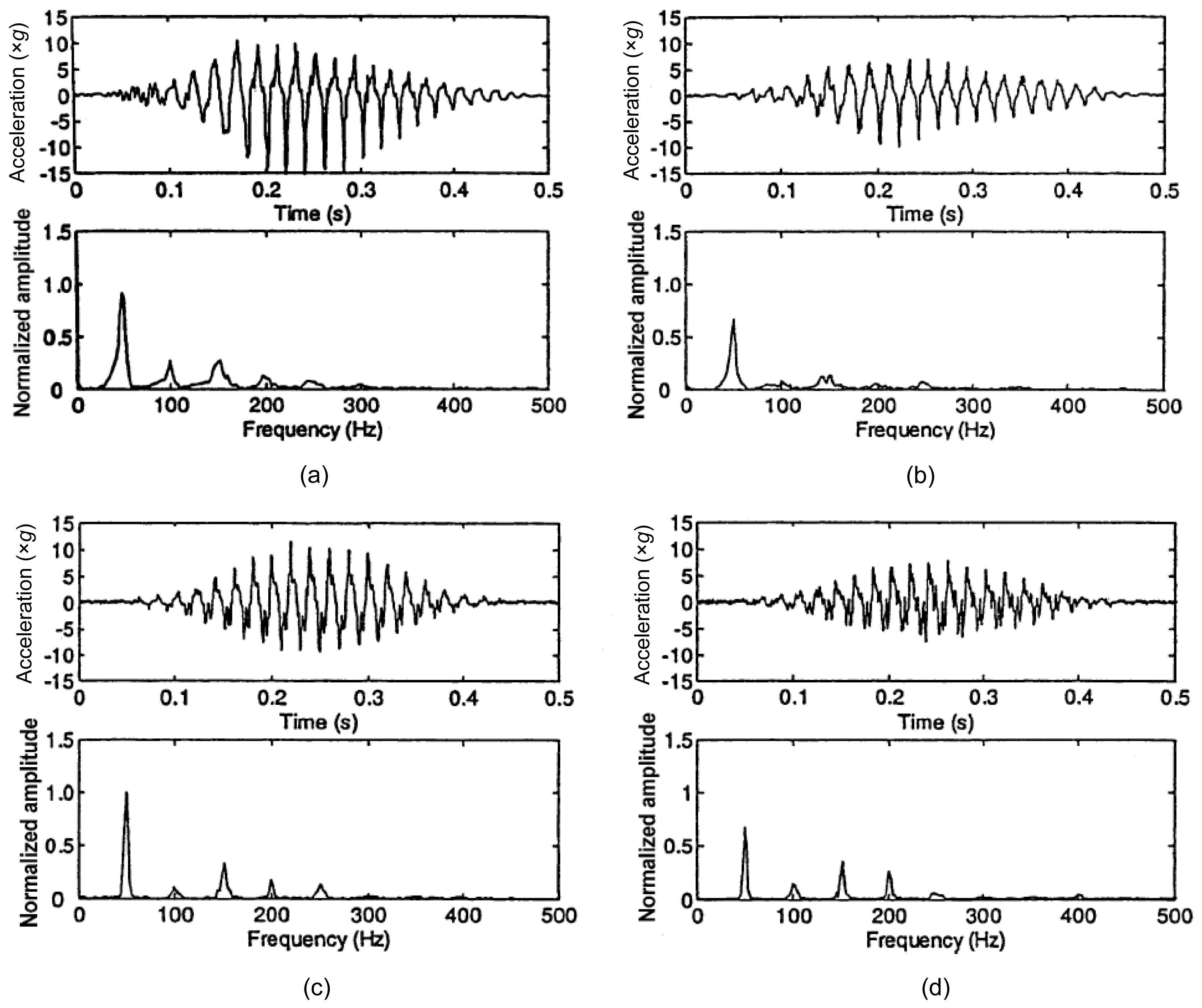
Fig. 26 shows some measured horizontal acceleration time histories in the X- and Y-direction together with their normalised amplitudes in the Fourier domain in the bi-axial shaking test. The base input accelerations (recorded by ACC-T-X and ACC-T-Y as shown in the figure) were 11.26g (0.28g prototype) and 7.77g (0.19g prototype) in the X-direction and Y-direction, respectively. The windowed sinusoid waveform applied in the Y-direction lagged the X-direction input signal by 90°. Recorded by the accelerometer near the crest, the peak acceleration in the X-direction increased by 45% at ACC4-X, which is higher than that measured in a corresponding uni-axial shaking test (Ng et al., 2004b). A similar trend of variations in the acceleration was also found in the Y-direction. The normalised spectral amplitudes of acceleration at the predominant frequency of 50 Hz decreased by about 9% in the X-direction but increased by about 4% in the Y-direction in the upper portion of the embankment.
Fig.26 Seismic acceleration history and Fourier amplitude spectrum in the bi-axial shaking test (Ng et al., 2004b) (a) ACC4-X; (b) ACC4-Y; (c) ACC-T-X; (d) ACC-T-Y
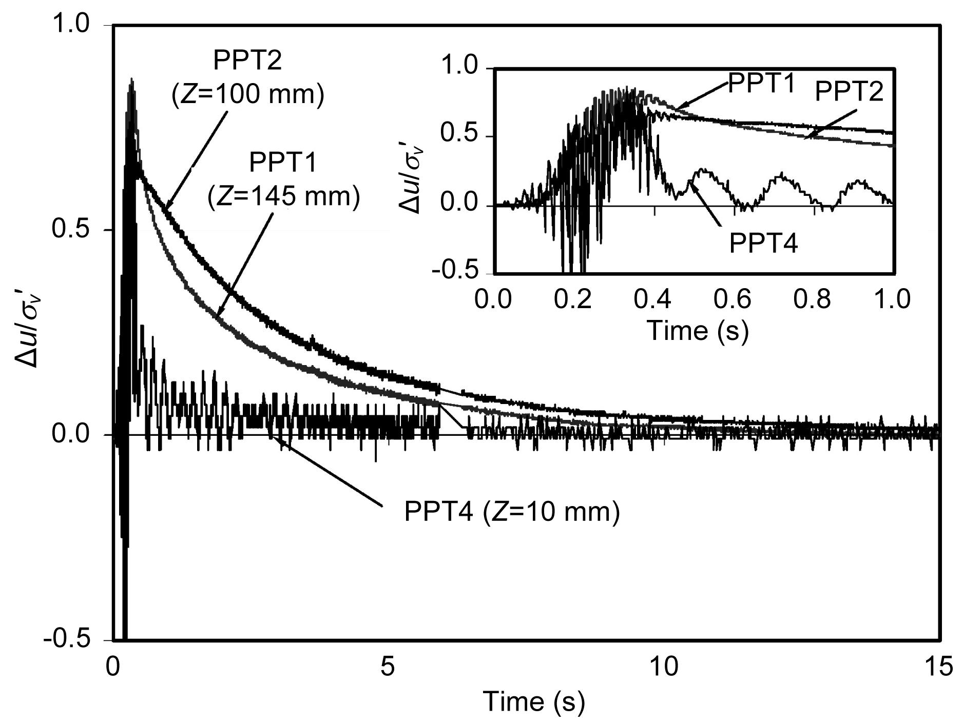
Fig. 27 shows the time history of the excess pore pressure ratios along the height of the model embankment during shaking. Peak acceleration occurred at about 0.25 s after the start of shaking. The maximum pore pressure ratio occurred at about 0.33 s at each of the three transducers (PPT1, PPT2, and PPT4). PPT1 and PPT2 recorded about the same maximum pore pressure ratio of 0.87, whereas PPT4 registered the smallest at 0.75. These measured values were less than the theoretical value of 1.0 for liquefaction, even though the pore fluid was correctly scaled in the test. The excess pore pressures dissipated to zero at about 12 s (6.8 min in prototype) after the start of shaking.
Fig.27 Measured excess pore water pressure ratios in the bi-axial shaking test M2D-0.3 (Ng et al., 2004b)
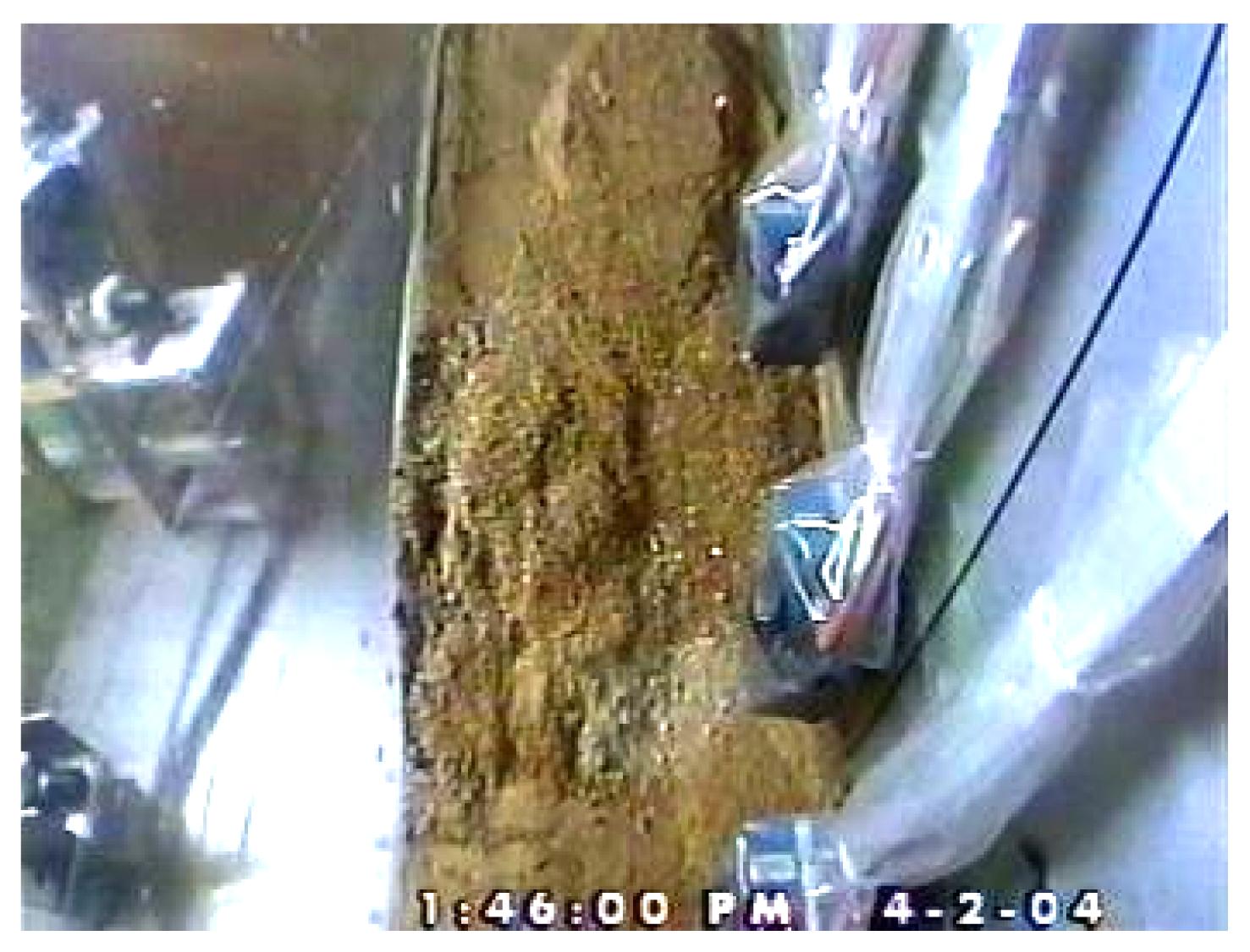
Fig. 28 shows a photograph of the model taken after the completion of a shaking test. The deformation profile for the slope was similar in both the uni-axial and bi-axial shaking tests. The observed profile of the deformed slope clearly illustrates that no liquefied flow and non-liquefied slide took place during the shaking. This suggests that loose CDG slopes are likely to be stable under the proposed design earthquake peak ground acceleration ranging from 0.08g to 0.11g in Hong Kong.
Fig.28 A typical profile of a loose fill slope after shaking (Ng et al., 2004b; 2007)
6.5. Inter-relationship between centrifuge modelling, numerical modelling, and field monitoring
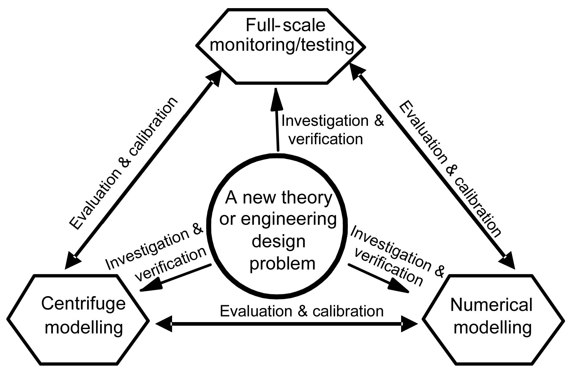
Apart from centrifuge modelling, two other major tools used for solving geotechnical problems are numerical modelling and field monitoring. Fig. 29 illustrates the inter-relationship between centrifuge modelling, numerical modelling, and full-scale field monitoring/testing. These three approaches are complementary with each other since no approach is perfect for every geotechnical and geo-environmental problem in terms of quality and reliability of result, time, and cost. They each have their own advantages and disadvantages.
Fig.29 Inter-relationship between centrifuge modelling, numerical modeling, and full-scale field monitoring/testing
Although both centrifuge tests and full-scale field tests can provide physical data, many numerical modellers suggest using full-scale field tests and case histories to calibrate their constitutive models and model parameters. This type of calibration can be very misleading since compensating errors are often overlooked (Fig. 30). For instance, field data are always subjected to many uncertainties because the actual ground conditions, anisotropy in terms of strength, stiffness and permeability, degree of saturation, soil homogeneity and boundary conditions are normally not known for sure. Any computed results, which “match” with observed and measured field behaviours, may be fortuitous resulting from compensating errors.
Fig.30 Concept of compensating errors
On the other hand, a mismatch between computed and measured data does not necessarily imply that either field measurements or numerical predictions are incorrect. As illustrated in Fig. 31, there is a missing link in the procedure of calibrating numerical models and model parameters using field data. Prior to calibrating constitutive models and model parameters against field data/case histories, a vital intermediate step (i.e., physical model tests, either at 1g or high g) is desirable and necessary to provide ‘known’ boundary and ground conditions and soil parameters for numerical modellers since any physical model tests are man-made. Uncertainties in material properties, ground conditions, and boundary conditions can be minimised or even eliminated. Ideally, any numerical tool should be calibrated against measured data from well-controlled physical model tests first (such as flume and centrifuge tests), before trying to use it to predict actual field behaviour.
Fig.31 A missing link for calibrating numerical models and model parameters with field data/case histories
7. Conclusions
This ZENG Guo-xi Lecture reports four examples of the use of the state-of-the-art geotechnical centrifuge at the HKUST to investigate and understand complex geotechnical problems. Based on the centrifuge model tests, the following conclusions can be drawn:
Building tilt often results from non-homogeneity of the ground or from adjacent underground constructions. One possible method for correction of building tilt is to extract soil (i.e., creating stress release) from the less settled side of a building. To verify the effectiveness of this method, in-flight vertical boring adjacent to an initially tilted building was simulated in the centrifuge, by using the advanced four-axis robotic manipulator at the HKUST. The centrifuge test demonstrated that vertical soil extraction could effectively reduce building tilt. The test results also suggested that to properly predict the correction of building tilt by vertical soil extraction, construction sequences and the plastic behaviour of soil should be taken into account.
Three-dimensional centrifuge model tests were conducted to investigate the effect of tunnel collapse on an adjecent exsiting tunnel. The centrifuge test results showed that due to tunnel collapse, bending moments at the crown, invert, and the right springline (close to the collapse) of the adjacent exising tunnel were increased by 60%, 28%, and 228%, respectively.
Influence of excavation on the capacity of a single pile installed underneath was investigated. Centrifuge tests reveal that pile capacity after excavation can either increase or decrease, depending on roughness of the soil-pile interface. For low friction piles (piles in non-dilatant geo-materials), ultimate shaft resistance reduces in proportion to the vertical stress relief resulting from excavation. On the other hand, the capacity of high friction piles (piles in dilatant geo-materials) increases (by about 39%) after excavation. This is because reduced stress level in the soil after excavation makes the rough soil-pile interface more dilatant. The dilation at the soil-pile interface increases horizontal stress acting on the pile, and hence increases the ultimate shaft resistance.
To further clarify and better understand “static liquifaction” and its importance in slope engineering, triaxial element tests and centrifuge model tests on loose fill slopes using gap-graded LB sand and a well-graded silty sand (i.e., CDG) were carried out. In the centrifuge test, static liquefaction/fluidisation of the loose LB sand fill slope due to a rising ground water table was successfully simulated. In contrast, only non-liquefied slide was observed in loose CDG fill slopes when they were subjected to a rising ground water table. The distinct difference between the observed centrifuge tests on the LB sand and CDG fill slopes may be attributed to the differences in the fine contents, gradation, and liquefaction potential of the two materials.
Apart from static tests, the dynamic response of a loose CDG fill embankment was also investigated using the bi-axial shaking table in the centrifuge at the HKUST. The bi-axial shaking test with a peak horizontal base acceleration of about 0.3g resulted in maximum excess pore water pressure ratios ranging from 0.75 to 0.87. No evidence of flow liquefaction was observed, indicating that loose CDG slopes are likely to be stable under the proposed design earthquake peak ground acceleration ranging from 0.08g to 0.11g in Hong Kong.
In addition to improving the understanding of complex geotechnical problems, well-controlled centrifuge tests can also provide high quality physical data to verify analytical and numerical methods. It is highly recommended that any numerical tool should be verified by well-controlled model tests (i.e., 1g or centrifuge tests) prior to predicting actual performce in the field, which often involves many more uncertainties than those in model tests.
Although geotechnical centrifuge is a powerful physical modelling tool for researchers and engineers, it has some limitations. For instance, it is not suitable for use in investigating soil creep, ageing, and compensation grouting for tunneling.
Acknowledgements
The author would like to thank Dr. Yi HONG, from HKUST, China for his assistance of formatting and proof-reading this paper.
Abbreviations of some institutions shown in Fig. 7 are given as follows (Table A1).
Abbreviations of some institutions shown in Fig. 7
Abbreviation
Institution
Country
Cambridge
Cambridge University
UK
ETH
Eidgenössische Technische Hochschule
Switzerland
HKUST
Hong Kong University of Science and Technology
Hong Kong, China
LCPC
Laboratoire Central des Ponts et Chaussées
France
NUS
National University of Singapore
Singapore
UC, Davis
University of California, Davis,
USA
UWA
University of Western Australia
Australia
WES
Waterways Experiment Station
USA
Zhejiang
Zhejiang University
China
References
[1] BS1377, 1990. Methods of Tests for Soils for Civil Engineering Purposes. British Standards Institution,London :
[2] Bucky, P.B., 1931. Use of models for the study of mining problems. American Institution of Mining and Metallurgical Engineers, 425:3-28.
[3] Cai, Z.Y., 2001. A Comprehensive Study of State-dependent Dilatancy and Its Application in Shear Band Formation Analysis. PhD Thesis, The Hong Kong University of Science and Technology,Hong Kong, China :
[5] Cheney, J.A., 1988. American literature review on geome-chanical centrifuge modelling 1931-1984. . Centrifuges in Soil Mechanics,Balkema, Rotterdam :77-88.
[7] DeJong, J.T., Frost, J.D., 2002. Physical evidence of shear banding at granular-continuum interfaces. , Proc. 15th ASCE Engineering Mechanics Conference, Columbia University, New York, NY, 8:8
[8] Fioravante, V., 2002. On the shaft friction modelling of non-displacement piles in sand. Soils and Foundations, 42(2):23-33.
[9] Garnier, J., Gaudin, C., Springman, S.M., 2007. Catalogue of scaling laws and similitude questions in geotechnical centrifuge modelling. International Journal of Physical Modelling in Geotechnics, 7(3):1-23.
[10] Hoek, E., 1965. The design of a centrifuge for the simulation of gravitational force fields in mine models. Journal of South African Institute of Mining and Metallurgy, 65(9):455-487.
[11] HSE (Health and Safety Executive), 2000. The collapse of NATM tunnels at heathrow airport. A Report on the Investigation by the Health and Safety Executive into the Collapse of New Austrian Tunnelling Method (NATM) Tunnels at the Central Terminal Area of Heathrow Airport on 20/21 October 1994. HSE Books,UK :
[12] Joseph, P.J., Einetein, H.H., Whiltman, R.V., 1988. A literature review of geotechnical centrifuge modelling with particular emphasis on rock mechanics. Massachusetts Institute of Technology,USA :
[13] Kimura, T., 1998. Development of geotechnical centrifuge in Japan. Proc, , Centrifuge, Tokyo, 23-32. :23-32.
[14] Kishida, H., Uesugi, M., 1987. Tests of the interface between sand and steel in the simple shear apparatus. Gotechnique, 37(1):45-52.
[15] Ko, H.Y., 1988. Summary of the state-of-the-art in centrifuge model testing. Centrifuge in Soil Mechanics, :11-28.
[17] Lei, G.H., Shi, J.Y., 2003. Physical meanings of kinematics in centrifuge modelling technique. Rock and Soil Mechanics, 24(2):188-193.
[18] Mindlin, R.D., 1936. Force at a point in the interior of a semi-infinite solid. Journal of Applied Physics, 7(5):195-202.
[19] Ng, C.W.W., 2005. Invited country report: failure mechanisms and stabilisation of loose fill slopes in Hong Kong. , Proceedings of International Seminar on Slope Disasters in Geomorphological/Geotechnical Engineering, Osaka, 71-84. :71-84.
[20] Ng, C.W.W., 2007. Liquefied flow and non-liquefied slide of loose fill slopes. , Proceedings of 13th Asian Regional Conference on Soil Mechanics and Geotechnical Engineering, Kolkata, Allied Publishers Private Ltd, :
[21] Ng, C.W.W., 2008. Invited special lecture: deformation and failure mechanisms of loose and dense fill slopes with and without soil nails. , Proceedings of 10th International Symposium on Landslides and Engineered Slopes, Xian, China, 159-177. :159-177.
[22] Ng, C.W.W., 2009. What is static liquefaction failure of loose fill slope. The 1st Italian Workshop on Landslides, Napoli, Italy, 1:91-102.
[23] Ng, C.W.W., Xu, G.M., 2003. In-flight centrifuge modelling of vertical relief boring technique. Chinese Journal of Geotechnical Engineering, (in Chinese),25(3):299-303.
[24] Ng, C.W.W., Van Laak, P., Tang, W.H., 2001. The Hong Kong geotechnical centrifuge. , Proceedings of 3rd International Conference on Soft Soil Engineering, Hong Kong, 225-230. :225-230.
[25] Ng, C.W.W., Yau, T.L.Y., Li, J.H.M., 2001. New failure load criterion for large diameter bored piles in weathered geomaterials. Journal of Geotechnical and Geoenvironmental Engineering, 127(6):488-498.
[26] Ng, C.W.W., Van Laak, P.A., Zhang, L.M., 2002. Development of a four-axis robotic manipulator for centrifuge modelling at HKUST. , Proceedings of International Conference on Physical Modelling in Geotechnics, St. Johns Newfoundland, Canada, 71-76. :71-76.
[27] Ng, C.W.W., Zhou, X.W., Chung, J.K.H., 2003. Centrifuge modelling of multiple tunnel interaction in shallow ground. , Proceedings of 13th European Conference on Soil Mechanics and Geotechnical Engineering, Prague, Czech Republic, 759-762. :759-762.
[28] Ng, C.W.W., Simons, N.E., Menzies, B.K., 2004. A Short Course in Soil-structure Engineering of Deep Foundations, Excavations and Tunnels. Thomas Telford,London :424
[29] Ng, C.W.W., Li, X.S., Van Laak, P.A., 2004. Centrifuge modelling of loose fill embankment subjected to uni-axial and bi-axial earthquakes. Soil Dynamics and Earthquake Engineering, 24(4):305-318.
[30] Ng, C.W.W., Pun, W.K., Kwok, S.S.K., 2007. Centrifuge modelling in engineering practice in Hong Kong. , Geotechnical Division Annual Seminar, The Hong Kong Institution of Engineers, Hong Kong, 55-68. :55-68.
[31] Ng, C.W.W., Boonyarak, T., Man, D., 2013. Three-dimensional centrifuge and numerical modeling of the interaction between perpendicularly crossing tunnels. Canadian Geotechnical Journal, 50(9):935-946.
[32] Ng, C.W.W., Shi, J.W., Hong, Y., 2013. Three-dimensional centrifuge modelling of basement excavation effects on an existing tunnel in dry sand. Canadian Geotechnical Journal, 50(8):874-888.
[33] Panek, L.A., 1949. Design of safe and economical structures. Transactions of the American Institute of Mining and Metallurgical Engineers, 181:371-375.
[34] Ramberg, H., 1968. Instability of layered systems in the field of gravity, I. Physics of the Earth and Planetary Interiors, 1(7):427-447.
[35] Shen, C.K., Li, X.S., Ng, C.W.W., 1998. Development of a geotechnical centrifuge in Hong Kong. , Proceedings of Centrifuge, Tokyo, 13-18. :13-18.
[37] Terracina, F., 1962. Foundations of the Leaning Tower of Pisa. Gotechnique, 12(4):336-339.
[38] Zhang, M., 2006. Centrifuge Modelling of Potentially Liquefiable Loose Fill Slopes with and without Soil Nails. PhD Thesis, The Hong Kong University of Science and Technology,Hong Kong, China :
[39] Zhang, M., Ng, C.W.W., 2003. Interim factual testing report I-SG30 & SR30. The Hong Kong University of Science and Technology,Hong Kong, China :
[40] Zhang, M., Ng, C.W.W., Take, W.A., 2006. The role and mechanism of soil nails in liquefied loose sand fill slopes. , Proceedings of 6th International Conference Physical Modelling in Geotechnics, Hong Kong, 391-396. :391-396.
[41] Zheng, G., Peng, S.Y., Diao, Y., 2010. In-flight investigation of excavation effects on smooth single piles. , Proceedings of 7th International Conference on Physical Modelling in Geotechnics, 847-852. :847-852.
[42] Zheng, G., Peng, S.Y., Ng, C.W.W., 2012. Excavation effects on pile behaviour and capacity. Canadian Geotechnical Journal, 49(12):1347-1356.
Open peer comments: Debate/Discuss/Question/Opinion


Open peer comments: Debate/Discuss/Question/Opinion
<1>