Similar articles

Abstract: To estimate the motion parameters of a moving target before its passing by the closest point of approach (CPA) point in a low frequency analyzing and recording (LOFAR) field, an error-free theoretical method based on the joint measurement of target radiated noise’s amplitude and frequency was presented. First, the error-free theoretical equations for target characteristic frequency, absolute velocity, the CPA, and amplitude of the radiation noise were derived by three equal interval measured values of the target amplitude and frequency. Then, the method to improve the calculation accuracy was given. Finally, the simulation and experiments were conducted in the air and showed the correctness of this method. By using one single piece of LOFAR, this method can calculate four target parameters and the relative error of each estimated parameter is less than 10%.

低频分析和记录场合基于幅度和频率联合测量的目标定位方法

研究目的：针对低频分析和记录（LOFAR）使用场合，利用目标的幅度和频率信息来解算目标运动要素。
创新要点：利用目标幅度和频率信息，推出无误差的目标特征频率、绝对速度、最接近点距离、辐射幅度等四个参量理论公式，并得到解算目标运动要素的优化方法。
研究方法：1.用计算机进行无误差的理论验证仿真，并在有噪声的影响下，验证算法的正确性；2.在空气中，使用汽车模拟目标的运动，用麦克风采集汽车运动的多普勒信号（见图2），验证算法的工程有效性和正确性。
重要结论：1.使用三次等间隔采样的目标幅度和频率信息，即可无误差地解算出目标特征频率、绝对速度、最接近点距离、辐射幅度等四个参量；2.使用优化后的算法，经实际空气实验验证，使用单个LOFAR传感器即可解算出目标的四个参量，且四个参量的估计相对误差小于10%。

关键词：低频分析和记录（LOFAR）；最接近点；多普勒频移；传播损失

1.  Introduction

 Low frequency analyzing and recording (LOFAR) is a very important application in the passive measurement field. Generally, LOFAR with no directivity can only passively receive radiated noise of the target. Line spectrum information contained in the noise is recorded and processed to calculate the motion parameters of the target. With characteristics of low cost, small volume, light weight, etc., the LOFAR is applied widely in various fields, for example, underwater target localization (Wu and Sun, 1999; Ling and Wang, 2007).

 Methods with single pieces of LOFAR for target parameter estimation are as follows. The classical algorithm for LOFAR, namely algorithm of Doppler-closest point of approach (CPA) was proposed in (Tao 2009). Tao (2009) calculated the velocity of the target and CPA approximately by recording the two symmetrical target frequencies of the CPA point. An improved algorithm of the Doppler-CPA was also proposed in (Tao, 2009), where the calculation of the absolute velocity of the target and the CPA error-free theoretical formula were deduced by introducing time information. All the methods above can only be applied after the target passes by the CPA point, which is limited in use. The approximate calculation method of the target speed and CPA was presented in (Yu, 2011), which used any of the three point of frequency measurements and information of the change rate of the target line spectrum. Actually, the Doppler variation of the target is originally a slow process with noise. Therefore, using the rate of change to calculate the target motion parameters may cause some large errors.

 Target localization with joint multiple LOFAR is another active direction, such as the classical LOFAR FIX (LOFIX) principle and analysis of localization accuracy in (Hu et al., 2009), the classical hyperbolic fixing (HYFIX) principle and analysis of localization accuracy in (Sun et al., 2010). The passive range estimation was completed by using a vector sensor array (Li et al., 2012). The passive parameter estimation and its accuracy were analyzed from different aspects (Shang et al., 1985; Mao, 2001; Brian and Kam, 2002; Xue et al., 2005; Ma, 2007; Cockrell and Schmidt, 2010). To improve the accuracy of the target frequency measurement, some methods of image processing were applied in previous studies (Fan et al., 2002; Yang et al., 2010).

 This paper focuses on using a single piece of LOFAR. The radiated noise’s amplitude of the target at any time (not restricted to passing by the CPA necessarily) is collected by three types of equal intervals. The error-free calculation formulas for the four types of status information consisted of absolute velocity of the target, characteristic frequency of the target, the closest distance, and the absolute amplitude, are then derived.

2.  Measurement model

2.1.  Measurements of frequency

 As shown in Fig. 1, the target moves with speed v, and the CPA is D. The characteristic frequency of the line-spectrum is f _T, t_i is measure time, r_i is distance from LOFAR to target, and φ_i is the relative bearing between the moving forward direction of the target and LOFAR in the ith measurement, i=1, 2, 3.




 By the Doppler shift equation, the line-spectrum frequency of the detected target by using LOFAR is (Tao and Wang, 2008) (1) , where f_i is the ith measured target frequency, and c is the speed of sound.

2.2.  Measurements of amplitude

 LOFAR is mainly used for recording and processing the strong line spectrum in the noise radiated by the target. According to (Liu and Lei, 1993), the line spectrum noise mainly consists of mechanical noise and propeller noise in the background noise of the target. The frequency ranges from 10 Hz to 2000 Hz.

 Regarding the target as a point source, according to the spherical wave theory of sound propagation, the transmission loss is (2) , where α is the absorption coefficient. The first item of the transmission loss is extended loss, and the second item is sound absorption loss.

 The empirical formula of the low frequency band absorption coefficient which is derived from Liu and Lei (1993) is (3) .

 The absorption coefficient is 0.000279–0.12 in the frequency band of 10–2000 Hz. If the distance is 10 km, the extended loss will be 80 dB, and the maximum absorption loss is 1.2 dB. Therefore, the absorption loss can be ignored when the frequency is in the low band.

 Assuming that there are only extended loss and expansion of spherical waves, the amplitude data of the target noise which is received by LOFAR are (Liu and Lei, 1993) (4) , where p is the pressure of sound, and A is the amplitude of sound pressure which is equivalent to the unit distance from the target.

2.3.  Equation of observation

 As shown in Fig. 1, the frequency and amplitude of the target are measured and recorded at equal interval times t ₁, t ₂, and t ₃ (t ₂−t ₁=t ₃−t ₂=Δt). The measurement of frequency is shown in Eq. (1).

 The measurement of amplitude is (5) , where p_i is the signal amplitude of the target in the ith measurement, i=1, 2, 3. A _T is the absolute amplitude which is equivalent to the unit distance from the target. According to the geometric principle, (6) .

3.  Calculation of the target’s parameters

3.1.  Characteristic frequency

 Eq. (1) can be rewritten as (7) , and Eq. (5) can be rewritten as (8) , then (9) .

 Substituting Eq. (9) into Eq. (6), and substituting the measured values of t ₁, t ₂, and t ₃, we have (10) .

 Because f ₁, f ₂, f ₃ and p ₁, p ₂, p ₃ have been obtained, according to Eq. (10) the characteristic frequency f _T of the target can be resolved as follows: (11) .

3.2.  Absolute velocity

 According to the principle of trigonometric function and using the measured values of t ₁, t ₂, and Eq. (7)²+Eq. (8)²=1, we have (12) Eq. (12) can also be expressed in a matrix: (13) .

 The velocity v and D/A _T can be solved as f _T has been known.

3.3.  Closest point of approach (CPA)

 When f _T, v, and D/A _T have been known, tgφ_i can be calculated on the basis of Eq. (9). Then the closest point of approach D can be derived from Eq. (6) by use of the two values tgφ ₁ and tgφ ₂. Finally, the absolute amplitude A _T at the distance which is equivalent to the unit distance from the target can be resolved.

4.  Algorithm improvement

 Only three measured data have been used in the method mentioned above. To improve the calculation accuracy in practice, the best results can be obtained by using the statistical method with more data.

4.1.  Improvement of target characteristic frequency

 For the characteristic frequency of the target, the arithmetic average of multi-point calculation results f _T1, f _T2, …, f _Tn that can be obtained from Eq. (11) is used as the final characteristic frequency. (14) .

4.2.  Improvement of target velocity

 Using the multi-point data, Eq. (13) can be rewritten as (15) . For , , and , then in the least squares sense, there is (16) .

5.  Computer simulation

5.1.  Error-free simulation

 First of all, the correctness of the formula will be verified by use of the computer simulation without consideration of any error.

 We set the target speed of 5 m/s, characteristic line spectrum of 1000 Hz, radiation sound source level of 134 dB, and the equivalent voltage of 1 m away from the target A _T=501.90 V (which is calculated on the condition that the sensitivity of acoustic receiving transducer is −203 dB, and the gain of the preamplifier circuit is 120 dB).

 LOFAR is located in the origin of the coordinates, and the closest distance D to the target is 100 m, 1000 m, and 10000 m. Matlab is used as the simulation software. The sample rate of the frequency and amplitude is 1 Hz, sound speed is 1500 m/s, and time zero is set at the moment that the target passes by the CPA point (the CPA point in Fig. 1). The information of Doppler and amplitude of the targets which contain −300 s, −200 s, and −100 s is used for the calculation.

 The calculated results of the simulation model and sample data without errors are shown in Table 1.

 Because this algorithm is theoretically accurate and error-free, the calculation error depends entirely on the error of the calculation process. Matlab acted as the numerical simulation software due to its high calculation accuracy. In the actual process, the error of each calculated result can reach 10⁻¹⁴ orders of magnitude. Table 1 does not list all the significant figures as it is limited by the table size. As in the case of 1000.00 m, the actual calculated velocity is 4.99999999999998, and the distance is 1000.0000000000024. The correctness of this algorithm can be proved from the simulation results.

5.2.  Simulation with error

 Parameters of simulation with error are consistent with those of error-free simulation in section 5.1. The measurement error of frequency and amplitude is given below. Liu and Lei (1993) showed that in the deep sea the marine environment noise level is about 55 dB near the frequency of 1000 Hz, and the equivalent noise voltage is 0.0563 V (the transducer sensitivity is −203 dB, and the gain of the preamplifier circuit is calculated as 120 dB). In the simulation, the amplitude of the measured signal is given as follows: (17) , where p(k) is the magnitude of the signal at time k, r(k) is the distance from the target to the LOFAR at time k, and n _A is the Gaussian white noise with mean square error of 0.0536 V and with a mean of zero.

 At present, the detection of the frequency is mainly using an adaptive line spectrum enhancer, which can greatly improve the frequency measurement under the colored noise. Its measurement accuracy can reach 0.1 Hz, which is given by (18) , where f(k) is the measured value of the frequency at time k, f _T(k) is the real value of the target’s frequency at time k, and n _F is the Gaussian white noise with a mean square error of 0.1 and mean of zero.

 Eqs. (14) and (16) are applied when calculating the target parameters. The calculated results and the relative errors of the calculated results are shown in Table 2.




 As shown in Table 2, the calculated results are very accurate at close range (1000.00 m). The maximum relative error of distance is 2.91%, which can meet the actual requirements. Considering that we are only using a single piece of passive LOFAR, such results are still satisfactory.

 The error increases dramatically at far distance, e.g., in the case of 10000.00 m, the calculated error of the velocity is up to 26.60%. The main reason is that the variation of the target’s frequency and amplitude is reduced with the increasing distance, and the variation is almost the same as that of the amplitude of the noise. Therefore, the calculated error is very large, and may even result in a singular matrix which cannot be calculated.

6.  Experiment in the air

6.1.  Principle of the experiment

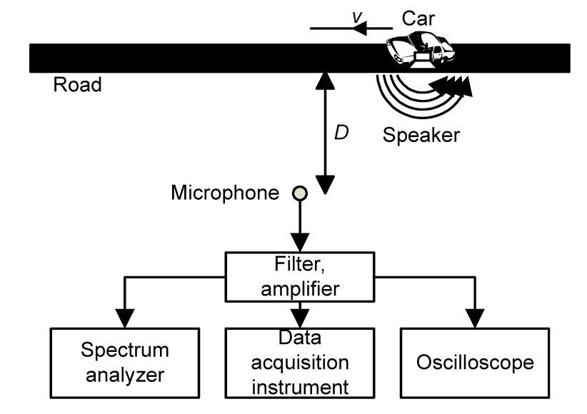
 A straight road was selected to be the experiment site, and a car was used to simulate the moving target with high-speed. The experimental equipment was divided into two parts: signal generation and acquisition. The car was used as the carrier of the signal generator which can produce a single frequency signal. The signal through a power amplifier would drive the high-power speaker to simulate the target with a single line spectrum. The signal acquisition part consisted of a high-sensitivity microphone, filter amplifier, spectrum analyzer, data logger, and oscilloscope. The microphone picked up the ambient noise in the air and the characteristic frequency of the target. After filtering and amplification, the data was finally collected and stored by the data acquisition instrument. The spectrum analyzer and oscilloscope as the monitoring devices were used to observe the noise signal in the frequency domain and time domain (Fig. 2).




 In the experiment (Fig. 2), the car traveling at a constant speed on the highway can simulate the targets which passed by the microphone, namely the CPA point at a uniform speed. The signal acquisition part collected the environmental noise and the target line spectrum which were stored by the data logger.

 The experiment content was mainly to change the different distances of the CPA (D in Fig. 2) and the car speed v, and then the collected sound data were used to calculate the frequency f of the signal, the absolute amplitude A, the speed v of the car, and the CPA distance D. The correctness of the algorithm and the effects of different factors on the algorithm will be verified in the experiment.

6.2.  Processing method

 The collected noise spectrum is a time domain signal. To estimate the frequency of each time accurately, the short-time Fourier transform method is used. In each fast Fourier transform (FFT), the length is to be 256 sampling points, the FFT overlap rate is 50%, and the length of the FFT algorithm is 1024. When the FFT of each time period is obtained, the frequency point with the maximum amplitude will be chosen as the measured frequency in this time period. The calculated frequency signal is to be handled by smooth filtering, namely using a 32-order finite impulse response (FIR) low-pass filter whose low-pass cut off frequency is 100 Hz.

6.3.  Experiment results and analysis

 In the process of the experiment, the microphone sensitivity is −45 dB, and the microphone frequency response band is 50 Hz–18 kHz. The gain of the amplifier is 60 dB, and the pass band frequency range of the filter is 0–20 000 Hz. The sampling rate of the data logger is 50 000 Hz. Four different CPAs are selected in the experiment, i.e., 7, 11.6, 15, and 20 m (due to the environmental limitation of the actual road, the maximum distance is 20 m). The speed of the car is respectively selected as 20, 40, 60, and 80 km/h. The frequency of the signal is 1000 Hz. The battery is chosen to be the energy source to drive the signal whose amplitude remains constant with the root mean square (RMS) of 15.55 V_RMS. The speed of sound in the air is taken as c=340 m/s while processing the data.

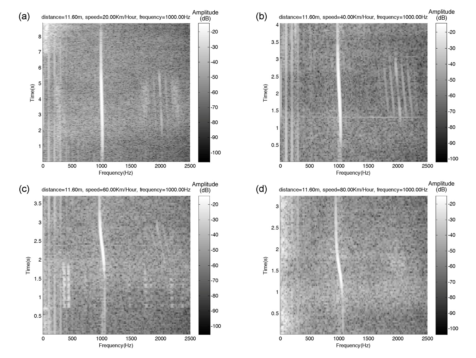
 Some typical processed results are shown in Fig. 3. Fig. 3 is the time-frequency cumulative results, in which the target passes by the CPA point whose distance is 11.60 m, the speed is respectively set as 20, 40, 60, and 80 km/h, and the characteristic frequency is 1000 Hz. The higher the brightness of the figure is, the greater the amplitude of the signal means. When the vehicle approaches, the frequency of the signal is greater than the actual frequency (1000 Hz), and the Doppler is positive. When the car departs, the frequency of the signal is decreasing, and the Doppler is negative.




 The turning points at the frequency curve indicate the time when the target passed by the CPA point. It can be seen that the change rate of the CPA point is greater when the speed of the vehicle is higher.

 There are totally 13 times valid processes in the entire experiment. The frequency and the amplitude of the signal are handled on the computer. The results are shown in Table 3.




 The experiment has achieved good results (Table 3). Most of the processes (except the experiment No. 6) estimate the motion parameters of the target well. The relative error of the calculated distance has an average value of 3.95% and the maximum value of 9.90%, while the relative error of the calculated frequency has an average value of 0.19% and the maximum value of 0.38%. The relative error of the calculated velocity has an average value of 2.85% and the maximum value of 4.77%, and the relative error of the calculated amplitude has an average value of 3.19% and the maximum value of 9.71%.

 According to the analysis of the experiment results, the closest distance has the greatest impact on the calculation error, which is consistent with the results of the computer simulation. The greater the distance is, the larger the calculation error will be. The most accurate estimated parameter is frequency, due to the frequency being stronger in anti-interference ability than other parameters. At the same time, there is no error propagation in the calculation process, when this method is directly used to measure the frequency. The estimation accuracy of velocity is higher than that of the distance and absolute amplitude, because the velocity is directly due to the Doppler frequency shift. The accuracy of the velocity will decrease, if the accuracy of the frequency is lower. The estimation accuracy of the closest distance and the absolute amplitude is the worst one. The distance calculation depends on the change of the frequency. When the distance is far, the relative velocity is reduced, and the change rate of the frequency decreases, which is equal to the reduction of the signal noise ratio (SNR). Therefore, the accuracy of the calculated results is reduced. Moreover, for the amplitude of the signal, the external interference is added directly to the amplitude information, leading to poor estimation accuracy. For example, in the experiment of No. 6, a heavy truck passed by, so some strong broadband interference was introduced in the vicinity of the low frequency band of 300–500 Hz at the time of 0.075 s–0.18 s. The strong interference, shown in Fig. 3c, resulted in the reduction of the calculation accuracy of the parameter.

7.  Conclusions

 In this paper, radiated noise’s amplitude information of the target was added to the parameter calculation process of LOFAR firstly. In theory, the error-free formulas were derived by using the amplitude and frequency information of the target, through any three equal interval measurements. Four important parameters, that is the speed of the target, the closest distance, characteristic frequency, and absolute amplitude, were obtained.

 The method does not need to overcome the disadvantages of the previous methods. The calculation is completed without the requirement of the CPA point. It improves the calculation speed and efficiency of the LOFAR, and makes the tactics more flexible. Moreover, it is an error-free method in theory, and has important theoretical significance in the algorithm research of the LOFAR fields.

 The simulation and experimental results in air show the validity of the method. Relative error of each estimated parameter is less than 10%. Moreover, this method only uses one single piece of LOFAR, with the accurate estimation of the target distance, speed, frequency, and amplitude at close range. Hence, it has a very good application prospects for many engineering fields, such as road speed measurement, namely using a single microphone to measure the speed of a vehicle and amplitude level of the noise. Further research will focus on the case of how to improve the estimation accuracy of the target parameter over a long distance.

---

* Project supported by the National Natural Science Foundation of China (No. 51209173)